source(here::here("R", "alpha_diversity.R"))
source(here::here("R", "beta_diversity.R"))
library(phyloseq)
library(ggplot2)
library(factoextra)
library(vegan)
library(permute)betadiv_LR
1. Preparing R Session
1.1 Libraries
1.2 Check if you are in the right place
you have to be ANF2025/course-material-main
getwd()[1] "/Users/marcgarel/OSU/MIO/2026/Projet_2026/Formation_OMIC_2026/formation-metabarcoding-long-read/scripts"1.3 Output repertory position
output_beta <- here::here("outputs", "beta_diversity")
if (!dir.exists(output_beta)) dir.create(output_beta, recursive = TRUE)
output_beta
[1] "/Users/marcgarel/OSU/MIO/2026/Projet_2026/Formation_OMIC_2026/formation-metabarcoding-long-read/outputs/beta_diversity"1.4 Load the physeq object in R
physeq <-readRDS(here::here("data","asv_table","physeq.rds"))1.5 Rebuild the physeq_rar object in R
set.seed(123)
#re run subsampling if physeq_rar does not exist anymore
physeq_rar <- phyloseq::rarefy_even_depth(physeq, rngseed = TRUE)
`set.seed(TRUE)` was used to initialize repeatable random subsampling.Please record this for your records so others can reproduce.Try `set.seed(TRUE); .Random.seed` for the full vector...28OTUs were removed because they are no longer
present in any sample after random subsampling...2. Data processing and filtering
Data processing and filtering were performed to remove low-quality and low-abundance features before downstream analyses such as CLR transformation and PCA.
2.1 Data matrix preparation for analysis
#Get matrix otu_table
X <- as(otu_table(physeq), "matrix")

#lines = samples ; column = taxa
if (taxa_are_rows(physeq)) { X <- t(X) }
#See by yourself
#head(X)
2.2 Check global sparsity
No universal rules BUT :
< 70% zeros → generally acceptable
70–90% zeros → common in microbiome, but caution is needed
> 90% zeros → very sparse, filtering is usually recommended
#Zero proportion by  taxa
zero_rate_global <- sum(X == 0) / length(X)
zero_rate_global
[1] 0.6057Conclusion about this score?
2.3 Remove very sparse taxa : Keep taxa with < 90% zeros
# For each column (taxa), count the number of zeros and divide by the total number of rows (sample)
zero_rate <- colSums(X == 0) / nrow(X)
#recupere taxa VRAI/FAUX qui remplisent cette condition
keep_taxa <- zero_rate < 0.90
#Extrait condition ok
X_f <- X[, keep_taxa, drop = FALSE]

zero_rate_new <- sum(X_f == 0) / length(X_f)
zero_rate_new
[1] 0.4795Is this step necessary ?
2.4 Change zero values by CZM : Count Zero Multiplicative
Zero values were replaced using the Count Zero Multiplicative (CZM) method. CZM replaces zeros and adjusts other values to keep the relative proportions, allowing log-based transformations such as CLR to be applied.
Replace zeros using CZM : Input must be (data.frame or matrix) : rows = samples & cols = taxa
tmp <- zCompositions::cmultRepl(
  X_f,
  method = "CZM",
  label = 0, #here: replace all 0 values
  z.warning = 1 #Display warnings related to zero values or issues during transformation
)
No. adjusted imputations: 1 #See by yourself
#head(tmp)2.4.1 Checks
Checks were performed to confirm that the data are properly normalized (row sums ≈ 1) and contain no zero values.
#Important checks
rowSums(tmp)           # should be close to 1-> proportion
barcode13_combine_Q22 barcode14_combine_Q22 barcode17_combine_Q22
1 1 1
barcode18_combine_Q22 barcode19_combine_Q22 barcode20_combine_Q22
1 1 1
barcode21_combine_Q22 barcode22_combine_Q22 barcode23_combine_Q22
1 1 1
barcode24_combine_Q22
1 any(tmp == 0) # should be FALSE -> no more zero[1] FALSE2.5 CLR transformation
CLR transforms compositional data into log-ratios relative to the geometric mean, centering each sample around zero (linked to geometric mean property).
This removes the dependency between taxa and allows the use of standard statistical methods such as PCA.
#clr transformation
table_clr <- compositions::clr(tmp)
#Check
head(rowMeans(table_clr))  # should be ~ 0 for each sample
barcode13_combine_Q22 barcode14_combine_Q22 barcode17_combine_Q22
0.000000000000019318 0.000000000000030300 0.000000000000018736
barcode18_combine_Q22 barcode19_combine_Q22 barcode20_combine_Q22
0.000000000000000584 0.000000000000060599 -0.000000000000002022 Do you think this result is ok ?
2.6 Rebuild a phyloseq object only at the end
Replace original counts with CLR-transformed values
# Keep only the taxa retained after filtering (same as in X_f)
physeq_clr <- prune_taxa(colnames(X_f), physeq)

otu_table(physeq_clr) <- phyloseq::otu_table(
  t(as.matrix(table_clr)),  # convert from samples x taxa in taxa x samples & add new CLR otu_table
  taxa_are_rows = TRUE
)
#See
physeq_clr
phyloseq-class experiment-level object
otu_table() OTU Table: [ 581 taxa and 10 samples ]
sample_data() Sample Data: [ 10 samples by 16 sample variables ]
tax_table() Taxonomy Table: [ 581 taxa by 7 taxonomic ranks ]
refseq() DNAStringSet: [ 581 reference sequences ]head(physeq_clr@otu_table)OTU Table: [6 taxa and 10 samples]
taxa are rows
barcode13_combine_Q22 barcode14_combine_Q22 barcode17_combine_Q22
1002672 -4.0282 -2.038 -1.906
1002870 0.1864 -2.038 1.854
1006 2.1323 2.341 2.350
1008307 0.2734 -2.038 -1.906
1008392 0.9665 1.916 -1.906
102116 -0.0143 2.638 4.356
barcode18_combine_Q22 barcode19_combine_Q22 barcode20_combine_Q22
1002672 -2.877 -1.414 1.1356
1002870 1.464 -1.414 1.2692
1006 2.177 -1.414 1.8978
1008307 -2.877 -1.414 -3.0314
1008392 -2.877 -1.414 0.8637
102116 3.302 3.653 1.9413
barcode21_combine_Q22 barcode22_combine_Q22 barcode23_combine_Q22
1002672 -3.5855 -0.8991 -3.0705
1002870 -3.5855 -0.8991 1.2304
1006 0.8700 2.9823 3.1644
1008307 0.5335 -0.8991 -3.0705
1008392 1.1754 -0.8991 0.9427
102116 1.2014 3.2054 2.2268
barcode24_combine_Q22
1002672 0.5494
1002870 1.2108
1006 3.5910
1008307 -3.3464
1008392 1.2108
102116 1.51452.7 Taxonomic labeling and preservation of original identifiers
Taxonomic labels were generated from the tax_table to replace ASV identifiers (numeric) and improve interpretability for the figure generated in this TP. Original SPECIES IDs (NUMERICAL) were retained in the tax_table (taxid) to ensure traceability. Labels were validated to be unique and non-missing prior to updating taxa names.
2.7.1 Applied on physeq_clr object ( for clustering and ordination)
# Generate taxonomic labels (species-level with fallback)
new_labels <- make_tax_labels(physeq_clr, level = "species")

# Check that the number of labels matches the number of taxa
stopifnot(length(new_labels) == ntaxa(physeq_clr))
# Ensure no missing labels
stopifnot(!any(is.na(new_labels)))
# Ensure all labels are unique
stopifnot(anyDuplicated(new_labels) == 0)

# Store original taxIDs in tax_table
tax <- as.data.frame(tax_table(physeq_clr))
tax$taxid <- taxa_names(physeq_clr)
tax_table(physeq_clr) <- as.matrix(tax)

# Replace taxa names by taxonomic labels
taxa_names(physeq_clr) <- new_labels

#See
head(physeq_clr@otu_table)
OTU Table: [6 taxa and 10 samples]
taxa are rows
barcode13_combine_Q22
Candidatus_Pelagibacter_sp._IMCC9063 -4.0282
Gaiella_occulta 0.1864
Marivirga_tractuosa 2.1323
Maricurvus_nonylphenolicus 0.2734
Chitinispirillum_alkaliphilum 0.9665
Stanieria_cyanosphaera -0.0143
barcode14_combine_Q22
Candidatus_Pelagibacter_sp._IMCC9063 -2.038
Gaiella_occulta -2.038
Marivirga_tractuosa 2.341
Maricurvus_nonylphenolicus -2.038
Chitinispirillum_alkaliphilum 1.916
Stanieria_cyanosphaera 2.638
barcode17_combine_Q22
Candidatus_Pelagibacter_sp._IMCC9063 -1.906
Gaiella_occulta 1.854
Marivirga_tractuosa 2.350
Maricurvus_nonylphenolicus -1.906
Chitinispirillum_alkaliphilum -1.906
Stanieria_cyanosphaera 4.356
barcode18_combine_Q22
Candidatus_Pelagibacter_sp._IMCC9063 -2.877
Gaiella_occulta 1.464
Marivirga_tractuosa 2.177
Maricurvus_nonylphenolicus -2.877
Chitinispirillum_alkaliphilum -2.877
Stanieria_cyanosphaera 3.302
barcode19_combine_Q22
Candidatus_Pelagibacter_sp._IMCC9063 -1.414
Gaiella_occulta -1.414
Marivirga_tractuosa -1.414
Maricurvus_nonylphenolicus -1.414
Chitinispirillum_alkaliphilum -1.414
Stanieria_cyanosphaera 3.653
barcode20_combine_Q22
Candidatus_Pelagibacter_sp._IMCC9063 1.1356
Gaiella_occulta 1.2692
Marivirga_tractuosa 1.8978
Maricurvus_nonylphenolicus -3.0314
Chitinispirillum_alkaliphilum 0.8637
Stanieria_cyanosphaera 1.9413
barcode21_combine_Q22
Candidatus_Pelagibacter_sp._IMCC9063 -3.5855
Gaiella_occulta -3.5855
Marivirga_tractuosa 0.8700
Maricurvus_nonylphenolicus 0.5335
Chitinispirillum_alkaliphilum 1.1754
Stanieria_cyanosphaera 1.2014
barcode22_combine_Q22
Candidatus_Pelagibacter_sp._IMCC9063 -0.8991
Gaiella_occulta -0.8991
Marivirga_tractuosa 2.9823
Maricurvus_nonylphenolicus -0.8991
Chitinispirillum_alkaliphilum -0.8991
Stanieria_cyanosphaera 3.2054
barcode23_combine_Q22
Candidatus_Pelagibacter_sp._IMCC9063 -3.0705
Gaiella_occulta 1.2304
Marivirga_tractuosa 3.1644
Maricurvus_nonylphenolicus -3.0705
Chitinispirillum_alkaliphilum 0.9427
Stanieria_cyanosphaera 2.2268
barcode24_combine_Q22
Candidatus_Pelagibacter_sp._IMCC9063 0.5494
Gaiella_occulta 1.2108
Marivirga_tractuosa 3.5910
Maricurvus_nonylphenolicus -3.3464
Chitinispirillum_alkaliphilum 1.2108
Stanieria_cyanosphaera 1.51452.7.2 Applied on physeq_rar object (for future z-score heatmap)
# Generate taxonomic labels (species-level with fallback)
new_labels <- make_tax_labels(physeq_rar, level = "species")

# Check that the number of labels matches the number of taxa
stopifnot(length(new_labels) == ntaxa(physeq_rar))
# Ensure no missing labels
stopifnot(!any(is.na(new_labels)))
# Ensure all labels are unique
stopifnot(anyDuplicated(new_labels) == 0)

# Store original taxIDs in tax_table
tax <- as.data.frame(tax_table(physeq_rar))
tax$taxid <- taxa_names(physeq_rar)
tax_table(physeq_rar) <- as.matrix(tax)

# Replace taxa names by taxonomic labels
taxa_names(physeq_rar) <- new_labels
2.8 Compute final distance matrix for clustering & ordination analyses
La distance d’Aitchison est simplement la distance euclidienne calculée après transformation CLR.
physeq_clr_dist <- phyloseq::distance(physeq_clr, method = "euclidean")3. Hierarchical Clustering
A first step in many microbiome projects is to examine how samples cluster on some measure of (dis)similarity. There are many ways to do perform such clustering, see here. Since microbiome data is compositional, we will perform here a hierarchical ascendant classification (HAC) of samples based on Aitchison distance.
Hierarchical clustering involves several key steps.
First, a clustering method must be chosen (e.g., single, complete, UPGMA, Ward), as this choice influences the structure of the dendrogram.
Second, the overall quality of the clustering can be assessed, for example using the cophenetic correlation.
Finally, the number of clusters must be determined, for instance using the Silhouette method, and the dendrogram is then cut accordingly to define the final groups.
3.1 Different clustering with the four aggregation criterion
#Simple aggregation criterion
spe_single <- hclust(physeq_clr_dist, method = "single")
#Complete aggregation criterion
spe_complete <- hclust(physeq_clr_dist, method = "complete")
#Unweighted pair group method with arithmetic mean
spe_upgma <- hclust(physeq_clr_dist, method = "average")
#Ward criterion
spe_ward <- hclust(physeq_clr_dist, method = "ward.D")


# Retrieve sample names from metadata
labels_samples <- sample_data(physeq_clr)$Name

# Replace default sample labels (IDs) with sample names
spe_single$labels   <- labels_samples
spe_complete$labels <- labels_samples
spe_upgma$labels    <- labels_samples
spe_ward$labels     <- labels_samples

# Plot dendrograms using different clustering methods
par(mfrow = c(2,2))

plot(spe_single, main = "Single linkage")
plot(spe_complete, main = "Complete linkage")
plot(spe_upgma, main = "UPGMA")
plot(spe_ward, main = "Ward method")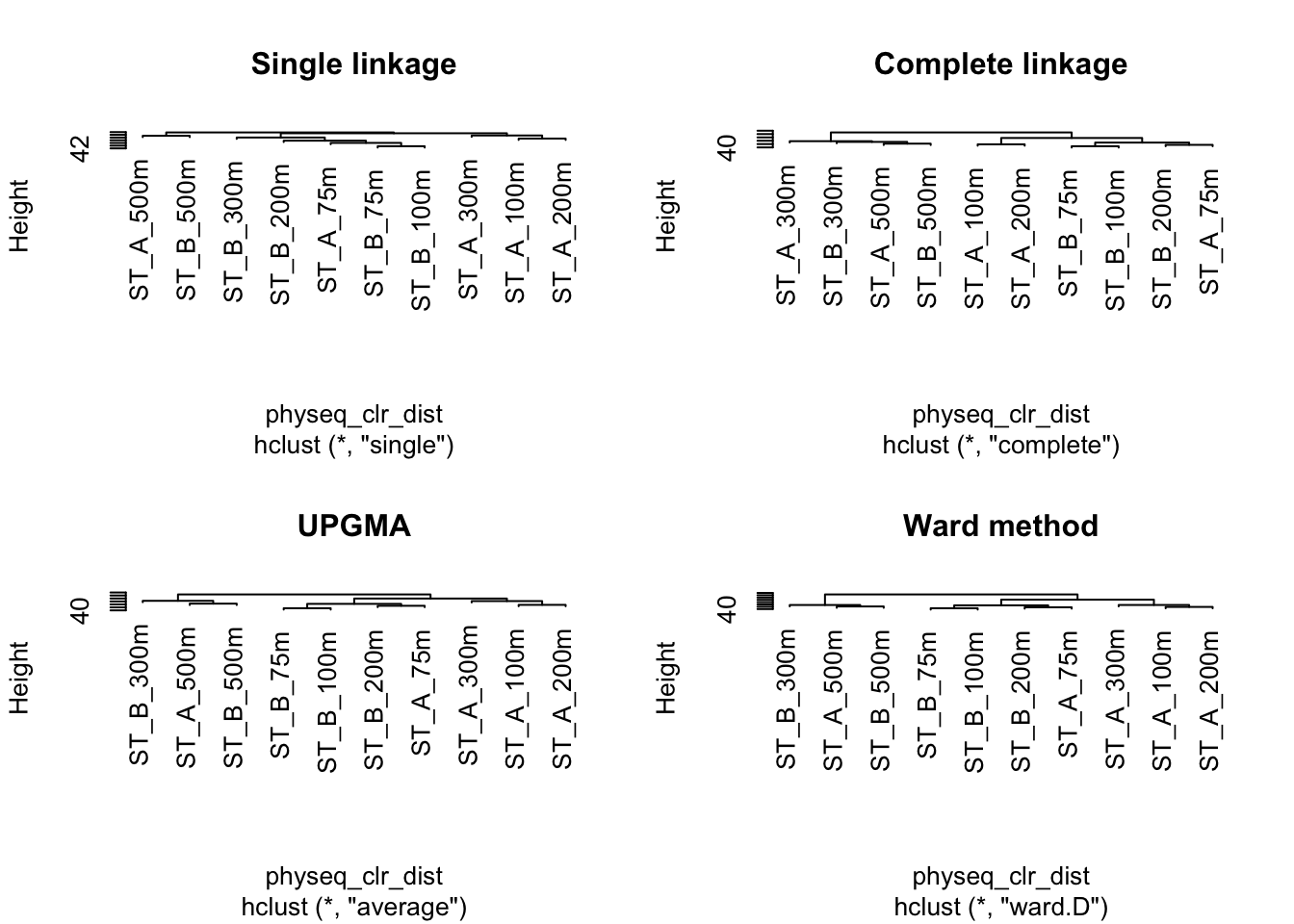
Clustering is not a statistical test but an exploratory method. The results depend on the distance measure and the clustering method used. Therefore, it is important to choose a method that fits the goal of the analysis.
3.2 Cophenetic Correlation
The cophenetic correlation measures how well a clustering represents the original distance between samples. The higher the value, the better the clustering. It Compares the original distance matrix with the distances obtained from the dendrogram.
A higher correlation indicates that the clustering better preserves the structure of the data.
Let us compute the cophenetic matrix and correlation of four clustering results presented above, by means of the function cophenetic() of package stats.
#Cophenetic correlation
spe_single_coph <- cophenetic(spe_single)
cor(physeq_clr_dist, spe_single_coph)
[1] 0.561spe_complete_coph <- cophenetic(spe_complete)
cor(physeq_clr_dist, spe_complete_coph)[1] 0.6586spe_upgma_coph <- cophenetic(spe_upgma)
cor(physeq_clr_dist, spe_upgma_coph)[1] 0.6574spe_ward_coph <- cophenetic(spe_ward)
cor(physeq_clr_dist, spe_ward_coph)[1] 0.6449Which clustering gives the most faithful representation of original distances? What about this score?
3.3 Looking for Interpretable Clusters
To determine the optimal number of clusters, we used the silhouette method. This approach evaluates how well each sample fits within its assigned cluster compared to other clusters. The optimal number of clusters corresponds to the highest average silhouette value ( (range: −1 to 1).
The higher the average silhouette value, the better the clustering.
Values > 0.5 indicate a strong structure, while values between 0.25 and 0.5 are considered acceptable, which is common in microbiome data.
factoextra::fviz_nbclust(
  otu_table(physeq_clr),
  FUNcluster = factoextra::hcut,
  method = "silhouette",
  hc_method = "complete", # the best one, step before
  hc_metric = "euclidean",
  stand = TRUE)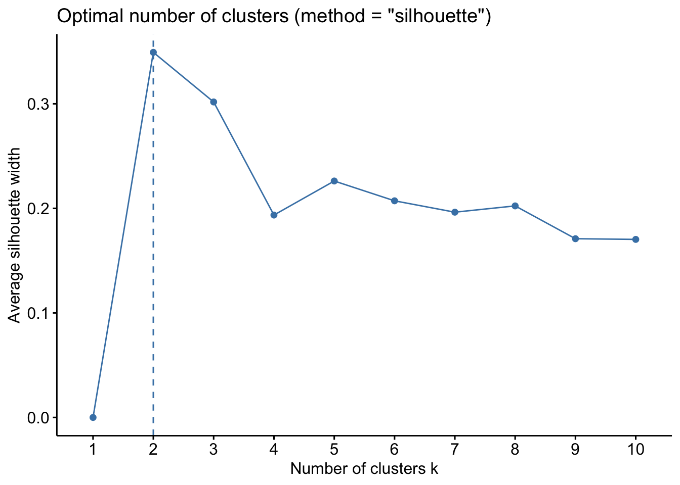
Conclusion about the optimal number of clusters and the robustness of this choice?
3.4 Hierarchical clustering dendrogram of samples
#apply
factoextra::fviz_dend(spe_upgma, k = 2,  # Cut in four groups
          cex = 0.4,                     # label size
          color_labels_by_k = FALSE,  # color labels by groups
          palette = "jco",               # Color palette see
          rect = TRUE, rect_fill = TRUE,
           rect_border = "jco",           # Rectangle color
          labels_track_height = 5,
          )+
  ggplot2::theme(legend.position = "none")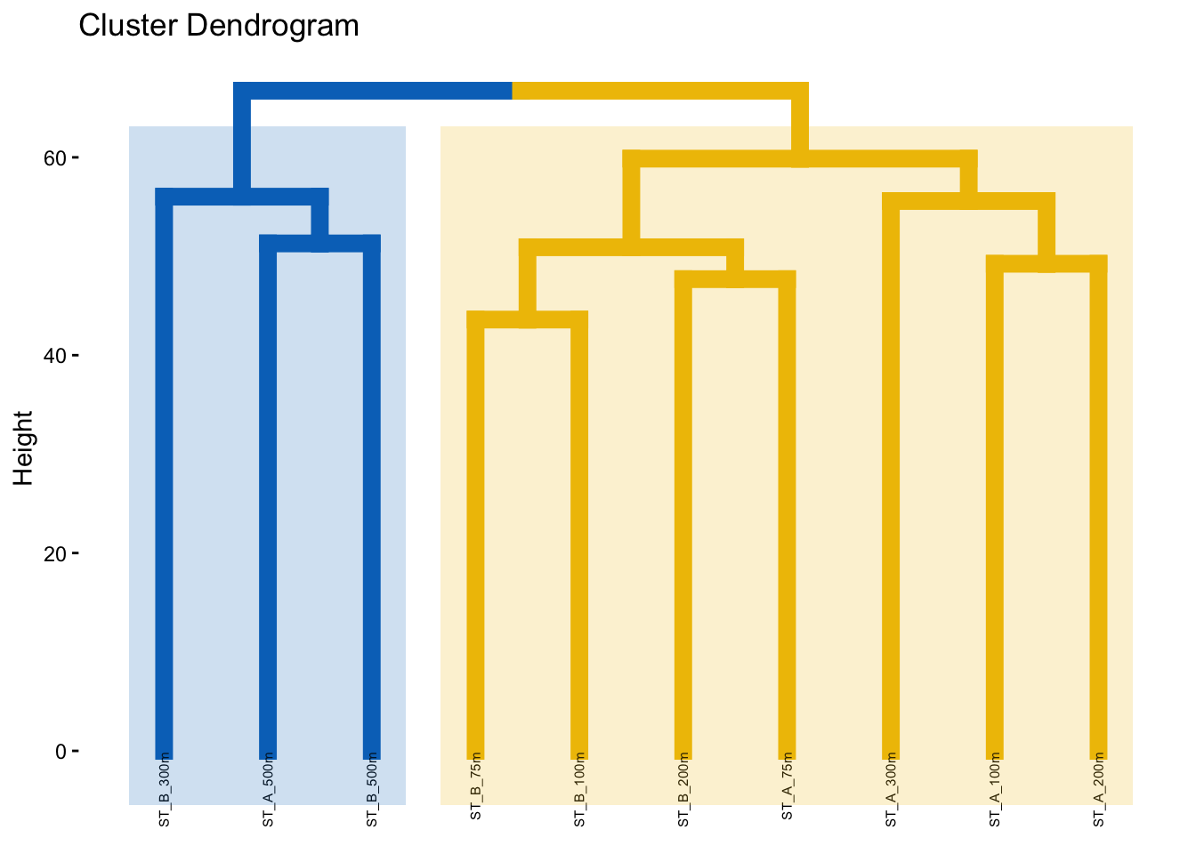
The height of the dendrogram represents the dissimilarity between samples or clusters, with higher values indicating greater differences.
Do the groups obtained makes sense?
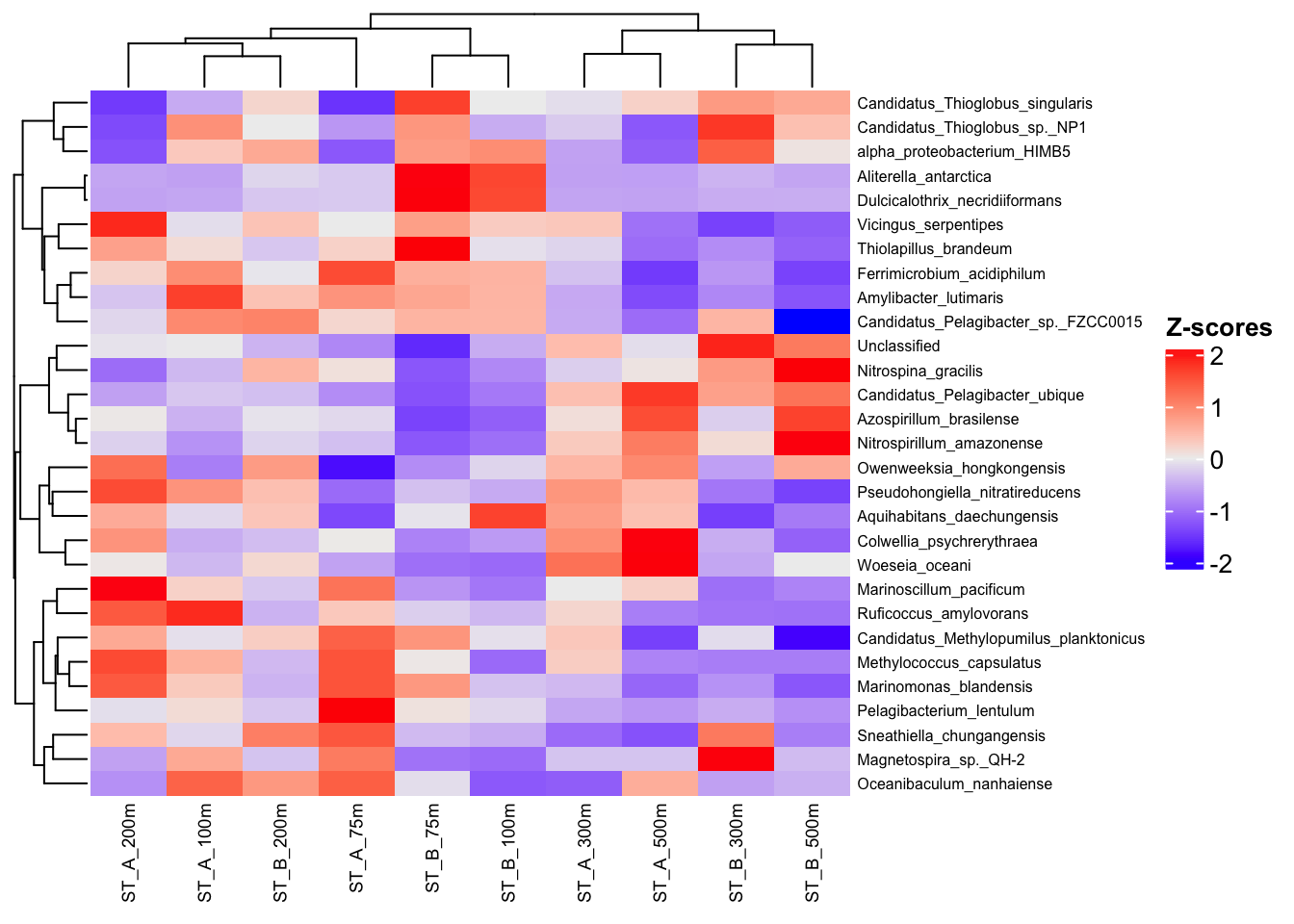
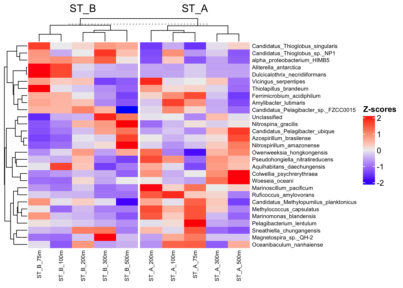
4. Clustering and Z-score Heatmap
Z-score heatmaps display normalized data, where values are centered around the mean (by row) and scaled by the standard deviation.
This transformation allows comparison of each sample to the average profile of the population.
A Z-score indicates how far a value deviates from the mean, expressed in units of standard deviation (SD).
We START here with physeq_rar NOT CLR transformation!!!!!
4.1 Select the top 30 species
Here we used species but of course you can do it on Family or genus taxonomic level!
#Transform Row/normalized counts in percentage: transform_sample_counts
pourcentS <- phyloseq::transform_sample_counts(physeq_rar, function(x) x/sum(x) * 100)
#Selection of top 30 taxa
mytop30 <- names(sort(phyloseq::taxa_sums(pourcentS), TRUE)[1:29])
#Extraction of taxa from the object pourcentS
selection30 <- phyloseq::prune_taxa(mytop30, pourcentS)
#See new object with only the top 30 species
selection30
phyloseq-class experiment-level object
otu_table() OTU Table: [ 29 taxa and 10 samples ]
sample_data() Sample Data: [ 10 samples by 16 sample variables ]
tax_table() Taxonomy Table: [ 29 taxa by 8 taxonomic ranks ]
refseq() DNAStringSet: [ 29 reference sequences ]Why selecting only top30 species ?
4.2 Proportion of total abundance explained by top taxa
sample_sums(selection30@otu_table)barcode13_combine_Q22 barcode14_combine_Q22 barcode17_combine_Q22
71.19 73.75 74.31
barcode18_combine_Q22 barcode19_combine_Q22 barcode20_combine_Q22
70.39 72.53 70.58
barcode21_combine_Q22 barcode22_combine_Q22 barcode23_combine_Q22
66.94 70.69 71.02
barcode24_combine_Q22
71.98 The top 30 taxa account for more than 70% of the total abundance, indicating that most of the information is retained after filtering.
# Abundance table: samples in rows, taxa in columns
selection30_sp <- as.data.frame(t(otu_table(selection30)), check.names = FALSE)

#Replace sample IDs by sample names
rownames(selection30_sp) <- sample_data(selection30)$Name

# Z-score normalisation by taxon
heat <- t(scale(selection30_sp))

# Check
head(as.data.frame(heat))
ST_A_300m ST_A_500m ST_B_75m ST_B_100m
Aquihabitans_daechungensis 0.78813 0.4299 -0.04777 1.683736
Thiolapillus_brandeum -0.17166 -1.0357 2.30663 -0.080715
Ferrimicrobium_acidiphilum -0.32275 -1.4864 0.59939 0.555480
Magnetospira_sp._QH-2 -0.30232 -0.3023 -0.98941 -1.058120
Sneathiella_chungangensis -1.05747 -1.2849 -0.37523 -0.488938
Candidatus_Thioglobus_singularis -0.09792 0.2495 1.70249 -0.003159
ST_B_200m ST_B_300m ST_B_500m ST_A_75m
Aquihabitans_daechungensis 0.37018 -1.4509 -0.9135 -1.361
Thiolapillus_brandeum -0.27398 -0.7628 -1.1266 0.249
Ferrimicrobium_acidiphilum -0.03732 -0.6740 -1.4205 1.609
Magnetospira_sp._QH-2 -0.30232 2.1025 -0.3710 1.141
Sneathiella_chungangensis 1.10295 1.1598 -0.8869 1.501
Candidatus_Thioglobus_singularis 0.21794 0.8181 0.6601 -1.551
ST_A_100m ST_A_200m
Aquihabitans_daechungensis -0.1373 0.6389
Thiolapillus_brandeum 0.1467 0.7492
Ferrimicrobium_acidiphilum 0.9507 0.2261
Magnetospira_sp._QH-2 0.6596 -0.5772
Sneathiella_chungangensis -0.1478 0.4776
Candidatus_Thioglobus_singularis -0.5085 -1.48774.3 Heatmap Z-score
Clustering are unsupervised approaches, as they rely only on the structure of the data and do not use external information.
In contrast, using column_split in a heatmap groups samples according to metadata (e.g., Station), which introduces a guided or supervised-like visualization to help interpret the results.
4.3.1 Unsupervised
ComplexHeatmap::Heatmap(
  heat,
  row_names_gp = grid::gpar(fontsize = 6), # species label size
  cluster_rows = TRUE, #species
  cluster_columns = TRUE, #clustering samples
  column_names_gp = grid::gpar(fontsize = 7),  # sample label size
  heatmap_legend_param = list(
    direction = "vertical",
    title = "Z-scores",
    grid_width = unit(0.5, "cm"),
    legend_height = unit(3, "cm")
  )
)
4.3.2 Supervised-like according the group Station
#Define a sample group
sample_group <- sample_data(selection30)$Station


ComplexHeatmap::Heatmap(
  heat,
  row_names_gp = grid::gpar(fontsize = 7), # species label size
  cluster_rows = TRUE, #species
  cluster_columns = TRUE, #samples
  column_split = sample_group,        # group samples by Station
  column_names_gp = grid::gpar(fontsize = 7),  # sample label size
  heatmap_legend_param = list(
    direction = "vertical",
    title = "Z-scores",
    grid_width = unit(0.5, "cm"),
    legend_height = unit(3, "cm")
  )
)
4.3.3 Add boxplots to visualize the distribution of taxon abundances across samples
Build the annotation box_plot
#create boxplot annotation for the distribution of abundances for each taxon
row_box <- ComplexHeatmap::anno_boxplot(
  t(selection30_sp), # transpose: taxa in rows, samples in columns
  which = "row", # apply boxplot to each row (each taxon)
  gp = grid::gpar(fill = "turquoise3")
)

# Add the boxplot annotation to the left side of the heatmap
left_anno <- ComplexHeatmap::rowAnnotation(
  Abundance = row_box, # name of the annotation
  width = grid::unit(3, "cm") # width of the annotation panel
)
4.3.4 Plot the final heatmap
ComplexHeatmap::Heatmap(
  heat,
  name = "Z-scores",
  row_names_gp = grid::gpar(fontsize = 7),
  column_names_gp = grid::gpar(fontsize = 7),
  cluster_columns = TRUE,
  cluster_rows = TRUE, #species
  column_split = sample_group,        # group samples by Station
  left_annotation = left_anno,
  heatmap_legend_param = list(
    direction = "vertical",
    title = "Z-scores",
    grid_width = grid::unit(0.5, "cm"),
    legend_height = grid::unit(3, "cm")
  )
)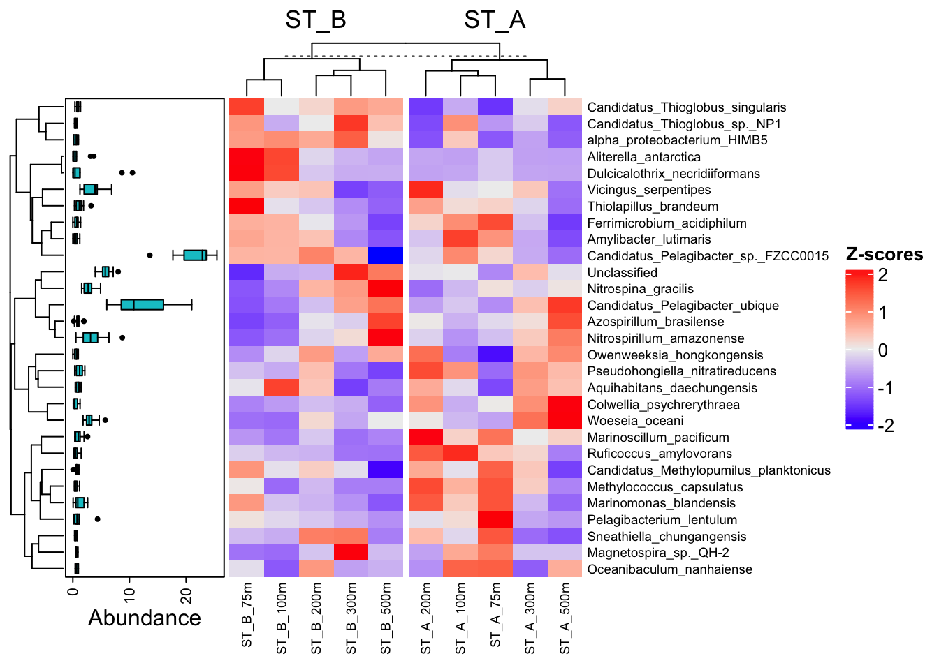
Conclusion ?
5. Indirect gradient analysis
Indirect gradient analysis (ordination) is used to explore patterns in ecological data. Unlike clustering, which identifies discrete groups, ordination describes continuous variation (gradients) in the data.
This makes ordination particularly suitable for ecological datasets, where communities are often structured along gradients rather than forming clear groups.
These methods reduce complex data into a few main axes that summarize the major trends. The first axis explains the largest part of the variation, followed by the next ones.
Common ordination methods include PCA, PCoA and NMDS.
These approaches are descriptive and are mainly used to visualize and interpret the structure of the data.
5.1 PCA on CLR-transformed data
Microbiome data are compositional, as they represent relative abundances that sum to a constant. This compositional nature makes standard Euclidean distance inappropriate when applied directly to raw data.
To address this issue, a centered log-ratio (CLR) transformation was applied. This transformation converts relative abundances into log-ratios, placing the data in a Euclidean space. PCA is based on Euclidean distance.
When applied to CLR-transformed data, this Euclidean distance corresponds to the Aitchison distance, which is appropriate for compositional data. Therefore, PCA on CLR-transformed data provides a meaningful representation of the structure of microbial communities.
5.1.1 Distance (Already calculated… just for remember)
physeq_clr_dist <- phyloseq::distance(physeq_clr, method = "euclidean")5.1.2 Get the intial otu_table of the physeq_clr object
table_clr_asv <- as.data.frame(otu_table(physeq_clr),  check.names = FALSE)
#See Identifiers
head(table_clr_asv)
barcode13_combine_Q22
Candidatus_Pelagibacter_sp._IMCC9063 -4.0282
Gaiella_occulta 0.1864
Marivirga_tractuosa 2.1323
Maricurvus_nonylphenolicus 0.2734
Chitinispirillum_alkaliphilum 0.9665
Stanieria_cyanosphaera -0.0143
barcode14_combine_Q22
Candidatus_Pelagibacter_sp._IMCC9063 -2.038
Gaiella_occulta -2.038
Marivirga_tractuosa 2.341
Maricurvus_nonylphenolicus -2.038
Chitinispirillum_alkaliphilum 1.916
Stanieria_cyanosphaera 2.638
barcode17_combine_Q22
Candidatus_Pelagibacter_sp._IMCC9063 -1.906
Gaiella_occulta 1.854
Marivirga_tractuosa 2.350
Maricurvus_nonylphenolicus -1.906
Chitinispirillum_alkaliphilum -1.906
Stanieria_cyanosphaera 4.356
barcode18_combine_Q22
Candidatus_Pelagibacter_sp._IMCC9063 -2.877
Gaiella_occulta 1.464
Marivirga_tractuosa 2.177
Maricurvus_nonylphenolicus -2.877
Chitinispirillum_alkaliphilum -2.877
Stanieria_cyanosphaera 3.302
barcode19_combine_Q22
Candidatus_Pelagibacter_sp._IMCC9063 -1.414
Gaiella_occulta -1.414
Marivirga_tractuosa -1.414
Maricurvus_nonylphenolicus -1.414
Chitinispirillum_alkaliphilum -1.414
Stanieria_cyanosphaera 3.653
barcode20_combine_Q22
Candidatus_Pelagibacter_sp._IMCC9063 1.1356
Gaiella_occulta 1.2692
Marivirga_tractuosa 1.8978
Maricurvus_nonylphenolicus -3.0314
Chitinispirillum_alkaliphilum 0.8637
Stanieria_cyanosphaera 1.9413
barcode21_combine_Q22
Candidatus_Pelagibacter_sp._IMCC9063 -3.5855
Gaiella_occulta -3.5855
Marivirga_tractuosa 0.8700
Maricurvus_nonylphenolicus 0.5335
Chitinispirillum_alkaliphilum 1.1754
Stanieria_cyanosphaera 1.2014
barcode22_combine_Q22
Candidatus_Pelagibacter_sp._IMCC9063 -0.8991
Gaiella_occulta -0.8991
Marivirga_tractuosa 2.9823
Maricurvus_nonylphenolicus -0.8991
Chitinispirillum_alkaliphilum -0.8991
Stanieria_cyanosphaera 3.2054
barcode23_combine_Q22
Candidatus_Pelagibacter_sp._IMCC9063 -3.0705
Gaiella_occulta 1.2304
Marivirga_tractuosa 3.1644
Maricurvus_nonylphenolicus -3.0705
Chitinispirillum_alkaliphilum 0.9427
Stanieria_cyanosphaera 2.2268
barcode24_combine_Q22
Candidatus_Pelagibacter_sp._IMCC9063 0.5494
Gaiella_occulta 1.2108
Marivirga_tractuosa 3.5910
Maricurvus_nonylphenolicus -3.3464
Chitinispirillum_alkaliphilum 1.2108
Stanieria_cyanosphaera 1.51455.2 PCA on CLR-transformed data with species-level annotation
A PCA is performed on a CLR-transformed OTU table (data-matrix or data-frame), where taxa (variables) are in rows and samples are in columns, as required by PCAtools.
Input = OTU table
Output = PCA object
Metadata = annotation des samples
5.2.1 PCA run
p <- PCAtools::pca(table_clr_asv, metadata = data.frame(sample_data(physeq_clr)))5.2.2 Structure of the PCA results object (p)
p is the object storing PCA results (scores, loadings, variance, etc)
p$variance → variance explained by each principal component
p$loadings → contribution of taxa (species) to each principal component (= coordinates by paired PC)
p$rotated → coordinates (scores) of the samples in the PCA space
p$metadata → sample information
#See by yourself
#p
5.2.3 Proportion of variance explained by principal components :p$variance
PC1 and PC2 represent the main patterns of variation in the taxonomic composition of the samples.
PCAtools::screeplot(p, axisLabSize = 18, titleLabSize = 22)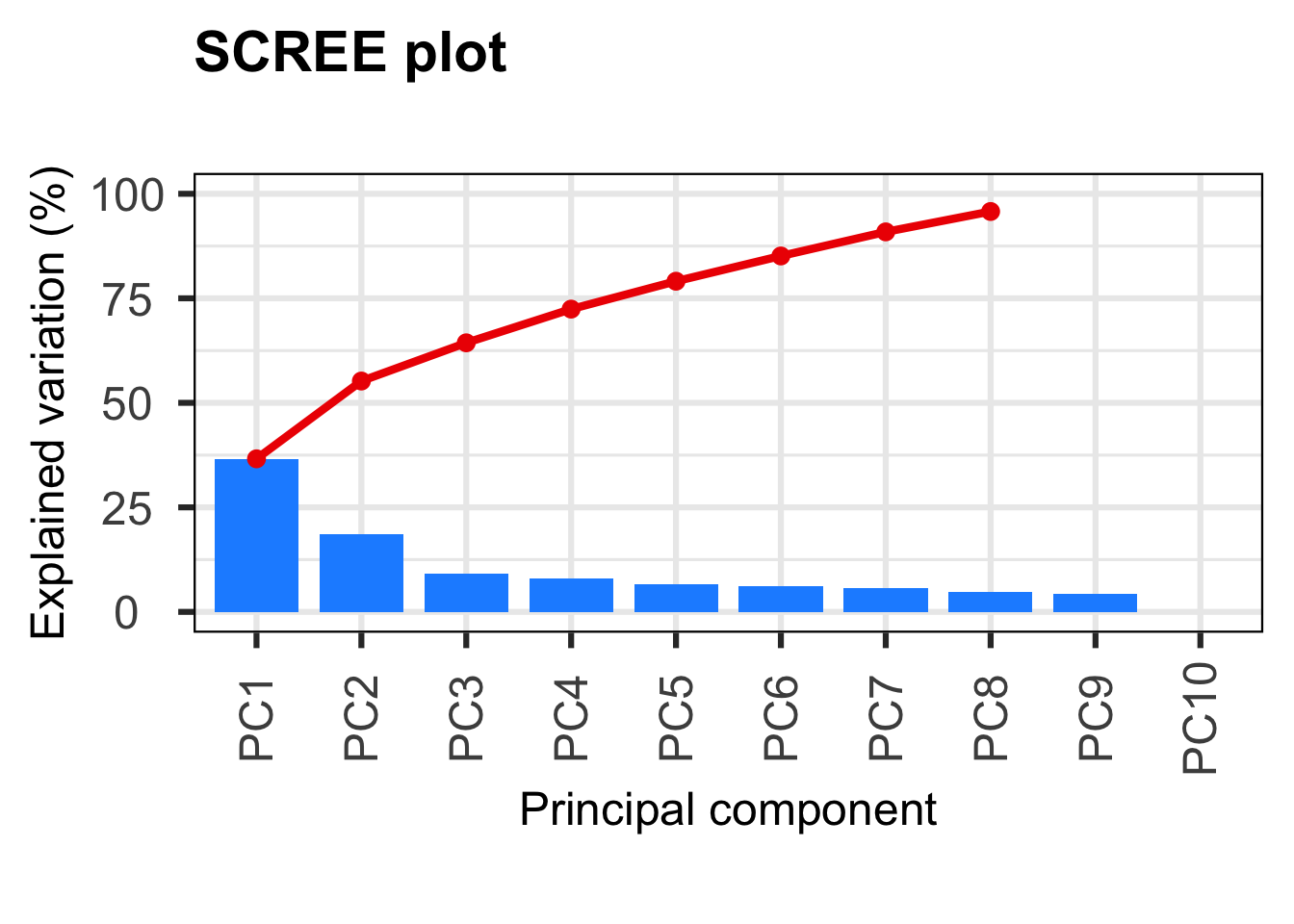
#variance explained by each PC
p$variance
PC1 PC2
36.611746069223841004713904112577438 18.603613629794342188006339711137116
PC3 PC4
9.138321131389746554418707091826946 8.063874398596423631602192472200841
PC5 PC6
6.669520228895077451625184039585292 6.043277389595059112537001055898145
PC7 PC8
5.761194930192225172049802495166659 4.874426547762269024133274797350168
PC9 PC10
4.234025674551086915187170234275982 0.000000000000000000000000000004258 5.2.4 Top taxa contributing to the first principal component (PC1) : p$loadings
This barplot shows the taxa with the highest contributions to PC1.Taxa with higher absolute loadings contribute more strongly to the variation captured by this axis, while the sign indicates their association with the positive or negative side of PC1.
Resume :
+ → taxon associated with the positive side of the axis
− → taxon associated with the negative side of the axis
value close to 0 → weak influence
high absolute value → strong contribution
See
head(p$loadings) PC1 PC2 PC3 PC4
Candidatus_Pelagibacter_sp._IMCC9063 0.005656 -0.001121 0.060850 -0.01844
Gaiella_occulta 0.051735 0.015963 0.065135 -0.03368
Marivirga_tractuosa 0.017333 0.036271 0.008182 0.01085
Maricurvus_nonylphenolicus -0.028241 -0.007712 -0.074671 -0.03631
Chitinispirillum_alkaliphilum -0.043553 0.050355 0.020726 0.01409
Stanieria_cyanosphaera 0.030091 -0.038364 -0.016617 0.03435
PC5 PC6 PC7 PC8
Candidatus_Pelagibacter_sp._IMCC9063 0.124004 -0.033380 -0.028261 0.002041
Gaiella_occulta -0.003579 -0.014592 0.034596 -0.029256
Marivirga_tractuosa 0.030569 0.031302 0.044416 -0.095656
Maricurvus_nonylphenolicus -0.030986 0.002167 0.018226 0.014340
Chitinispirillum_alkaliphilum 0.015831 0.035299 -0.008642 -0.025416
Stanieria_cyanosphaera 0.029355 -0.009067 -0.028150 0.024151
PC9 PC10
Candidatus_Pelagibacter_sp._IMCC9063 -0.01358 0.42859
Gaiella_occulta -0.05334 -0.26204
Marivirga_tractuosa -0.01108 0.50945
Maricurvus_nonylphenolicus 0.01313 0.01142
Chitinispirillum_alkaliphilum -0.03150 -0.12328
Stanieria_cyanosphaera -0.02493 0.06102Rapid plot of top15 contributor taxa
# Get PC1 contributions
loadings_PC1 <- data.frame( taxon = rownames(p$loadings), loading = p$loadings[, "PC1"])

# Keep top15 (by absolute value)
top15 <- loadings_PC1[order(-abs(loadings_PC1$loading)), ][1:15, ]

# Plot with positive/negative clearly visible
ggplot(top15, aes(x = reorder(taxon, loading), y = loading)) +
  geom_bar(stat = "identity") +
  coord_flip() +
  geom_hline(yintercept = 0) +   # ligne 0 pour voir + / -
  xlab(NULL) +
ylab("Loading (PC1)") 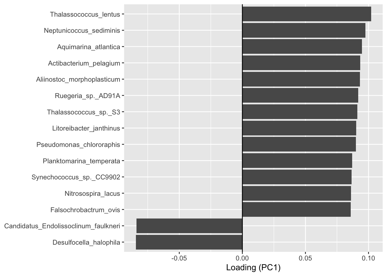
Do it for PC2!!!
5.2.5 PCA visualization of microbial communities : p$rotated
Separation of samples along an axis indicates differences in community composition.
Important : Values on PC1 and PC2 represent the coordinates of samples along the main axes of variation. These values have no direct units but reflect differences in taxonomic composition. The coordinate of a sample on a principal component is calculated as a weighted sum of its taxon abundances, using the corresponding loadings.
#See coordinates of samples
head(p$rotated)
PC1 PC2 PC3 PC4 PC5 PC6
barcode13_combine_Q22 -16.7517 21.3557 -5.7742 -14.5920 -12.984 -2.173
barcode14_combine_Q22 -28.5982 0.9787 -0.8931 28.8130 5.887 1.820
barcode17_combine_Q22 31.2650 -13.6914 -11.9775 -2.8695 -1.590 -8.593
barcode18_combine_Q22 31.3119 -22.5640 9.8662 7.6392 -11.167 -3.812
barcode19_combine_Q22 0.3748 -9.0532 -1.7368 -0.1654 -1.226 -8.786
barcode20_combine_Q22 -16.8771 -15.7416 26.5125 -13.8588 10.605 5.907
PC7 PC8 PC9 PC10
barcode13_combine_Q22 18.324 5.5324 -2.227 0.000000000000008537
barcode14_combine_Q22 8.389 2.0274 -6.437 0.000000000000008537
barcode17_combine_Q22 -2.462 -6.8068 -18.099 0.000000000000008537
barcode18_combine_Q22 10.062 -4.5610 12.857 0.000000000000008537
barcode19_combine_Q22 -12.012 23.0860 2.833 0.000000000000008537
barcode20_combine_Q22 1.535 -0.4129 -6.208 0.000000000000008537Plotting the PCA
#Plotting the PCA
PCAtools::biplot(
  p,
  lab = p$metadata$Name, #names from  column Name of metadata
  colby = "Station",    # color
  pointSize = 5,
  hline = 0, vline = 0,
  legendPosition = "right"
)
Ignoring unknown labels:
• fill : ""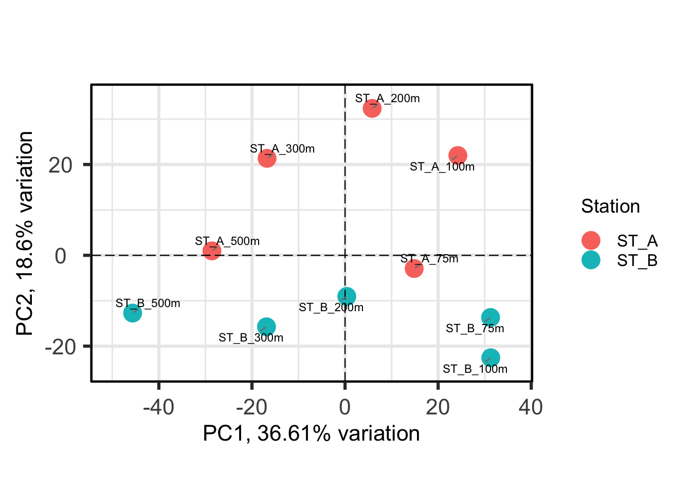
Each point represents a sample, and samples that are closer together are more similar in their microbial composition. Colouring by Station shows that samples from Station A and Station B tend to separate, indicating differences between communities.
What else can you see?
5.2.6 Determine the variables that drive variation among each PC
One benefit of not using a distance matrix, is that you can plot taxa “loadings” onto your PCA axes, using the showLoadings = TRUE argument. PCAtools allow you to plots the number of taxa loading vectors you want beginning by those having the more weight on each PCs. The relative length of each loading vector indicates its contribution to each PCA axis shown, and allows you to roughly estimate which samples will contain more of that taxon. https://www.bioconductor.org/packages/devel/bioc/vignettes/PCAtools/inst/doc/PCAtools.html
bp <- PCAtools::biplot(
  p,
    lab = p$metadata$Name,  #labels
  showLoadings = TRUE,  #  arrows representing taxa contributions
  boxedLoadingsNames = FALSE,   # do not draw boxes around taxa labels
  lengthLoadingsArrowsFactor = 1.5,  # adjust the length of loading arrows (scaling factor)
  sizeLoadingsNames = 3,  # size of taxa labels (text size)
  colLoadingsNames = 'red4',  # color of taxa labels
  ntopLoadings = 3,  # number of top contributing taxa to display by PC
  colby = "Station",
  hline = 0, vline = 0,
  legendPosition = "right"
)
bp
Ignoring unknown labels:
• fill : ""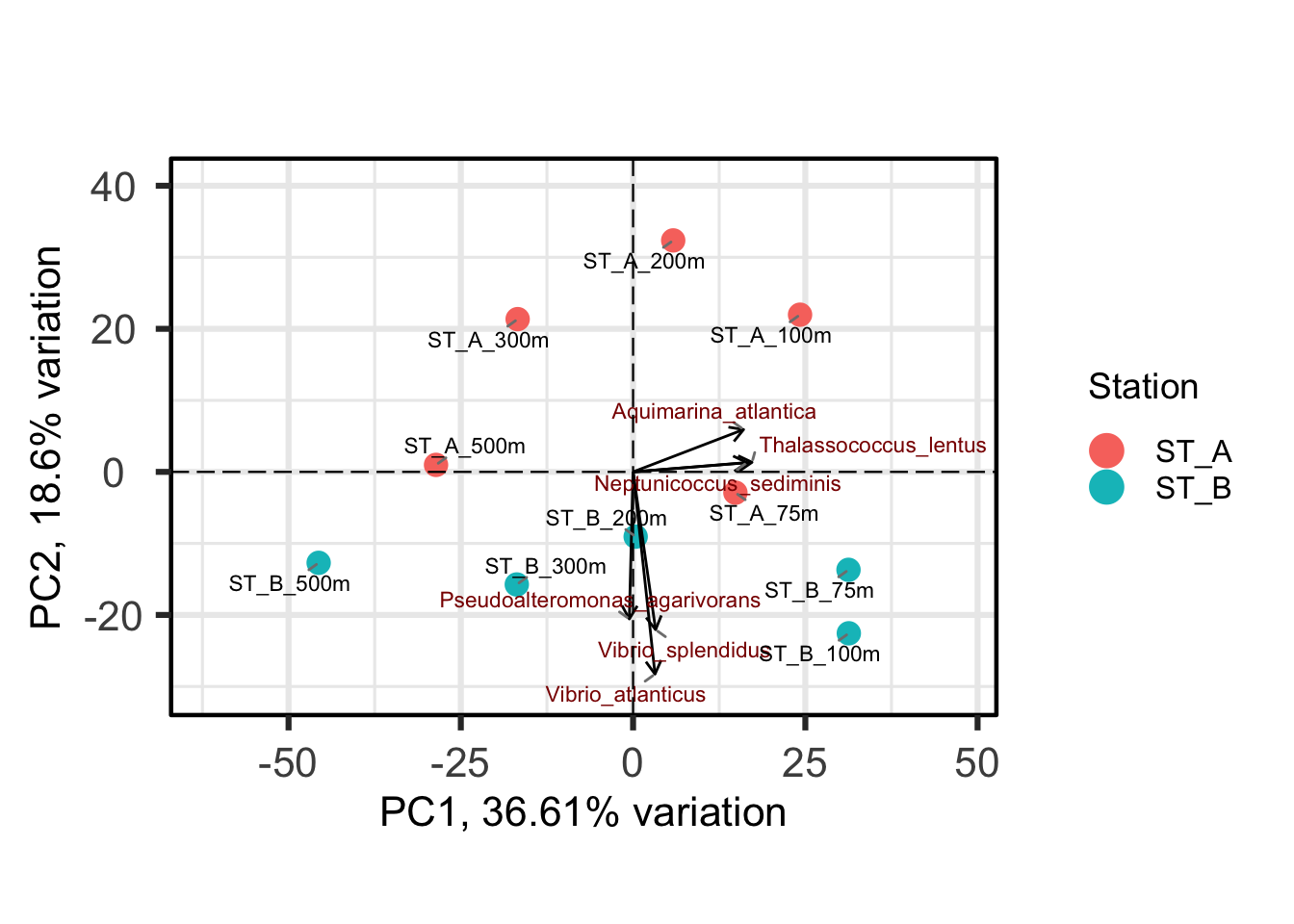
Conclusions about contributors of each PC axis?
PC1 and PC2 together explain around 55% of the total variance, indicating that the PCA plot captures a substantial part of the variation in the data, but not all of it.
Therefore, it can be important to explore additional principal components to better understand the remaining variation.
5.3 Exploration of additional principal components
Examining other combinations of principal components allows us to assess whether the observed patterns are consistent, and to detect additional structures that may not be visible in the PC1–PC2 plot.
PCA does not include metadata in its calculation (unsupervised method). By colouring samples using different variables (e.g., Station or Depth), we can explore possible explanations for the observed patterns and detect additional structures.
PCAtools::pairsplot(
  p,
  colby = "Station",
)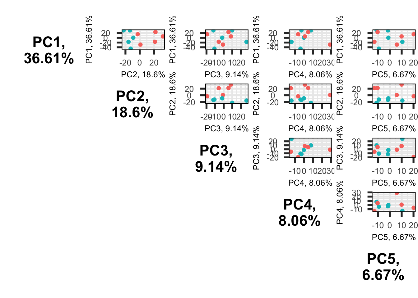
Conclusion?
5.4 Integration of environmental variables into PCA (envfit)
Environmental variables were fitted onto the PCA using the envfit method in order to assess their relationship with the main structure of the data.
This approach tests whether environmental variables are correlated with the biological gradients (mains contributors of PC1 & PC2) identified by the PCA, and therefore helps identify potential drivers (e.g. Depth, pH, NO3 etc) of community variation (= ecological interpretation).
Significant variables indicate a strong association with the ordination structure, while non-significant variables suggest a weak or no relationship. However, envfit only reveals CORRELATIONS and does not imply causation.
Exple: PC1 corresponds to a gradient of increasing or decreasing species abundances, which can then be interpreted using environmental variables.
5.4.1 Data extraction for envfit
#Extract PCA coordinates (samples) PC1 et PC2
ord <- p$rotated[, 1:2]

#Extract  variables from physeq@sam_data
env <- data.frame(sample_data(physeq))

#Select variables of interest
env_sub <- dplyr::select(env, O2, NO3, NH4, NO2, Salinity, pH, Turbidity, Pollutant)
# See
env_sub
O2 NO3 NH4 NO2 Salinity pH Turbidity Pollutant
barcode13_combine_Q22 128 18.5 0.94 0.11 38.32 8.06 1.8 9.44
barcode14_combine_Q22 82 27.6 0.57 0.05 37.88 7.98 2.1 9.33
barcode17_combine_Q22 232 2.4 0.44 0.04 38.41 8.12 1.5 9.30
barcode18_combine_Q22 221 4.2 0.41 0.13 38.05 8.03 2.3 9.30
barcode19_combine_Q22 171 10.8 0.52 0.17 37.72 7.95 1.9 9.00
barcode20_combine_Q22 129 18.1 0.86 0.09 38.28 8.10 2.0 8.84
barcode21_combine_Q22 82 28.5 0.43 0.03 37.95 8.01 1.7 8.57
barcode22_combine_Q22 228 2.0 0.40 0.06 38.10 7.92 2.2 9.74
barcode23_combine_Q22 208 4.8 0.69 0.11 37.83 8.08 1.6 9.83
barcode24_combine_Q22 166 9.9 0.98 0.19 38.36 8.00 1.8 9.665.4.2 Fitting environmental variables onto PCA (envfit)
# Set random seed to ensure reproducibility of permutation-based p-values
set.seed(123)

# Fit environmental variables onto the PCA ordination using envfit
env_fit <- vegan::envfit(
  ord,          # PCA coordinates (samples × axes)
  env_sub,      # selected environmental variables
  permutations = 999   # number of permutations for significance testing
)

#See
env_fit
***VECTORS

             PC1    PC2   r2 Pr(>r)
O2         0.995 -0.102 0.94  0.001 ***
NO3       -1.000 -0.026 0.93  0.001 ***
NH4       -0.201  0.980 0.54  0.082 .
NO2        0.445  0.895 0.28  0.325
Salinity   0.599  0.801 0.05  0.828
pH         0.977 -0.214 0.03  0.883
Turbidity  0.001 -1.000 0.12  0.654
Pollutant  0.562  0.827 0.81  0.002 **
---
Signif. codes:  0 '***' 0.001 '**' 0.01 '*' 0.05 '.' 0.1 ' ' 1
Permutation: free
Number of permutations: 999
env vectors : O2, NO3, NH4 etc
PC1 and PC2 : Coordinates of the env vector on the PCA axes
r2 : Strength of the correlation with the PCA
Pr>r : p-value -> probability of obtaining a correlation equal to or greater than the observed one under random permutations
What can you say ?
5.4.3 Extraction and preparation of PCA coordinates and environmental vectors
# Extract environmental vector scores
env_scores <- as.data.frame(env_fit$vectors$arrows)

# Identify significant vectors (p < 0.05)
significant <- env_fit$vectors$pvals < 0.05

# Keep only significant vectors
env_data <- env_scores[significant, , drop = FALSE]

# Store variable names
env_data$var <- rownames(env_data)
Give me the coordinates of NH4… and for Pollutant.
5.4.4 PCA ordination with fitted environmental variables (envfit)
# Rescale envfit vectors for display only
env_plot <- env_data
env_plot[, c("PC1", "PC2")] <- env_plot[, c("PC1", "PC2")] * 25

# Add environmental vectors to the PCA plot
bp +
  geom_segment(
    data = env_plot,
    aes(x = 0, y = 0, xend = PC1, yend = PC2),
    arrow = arrow(length = unit(0.1, "inches")),
    color = "blue",
    inherit.aes = FALSE
  ) +
  geom_text(
    data = env_plot,
    aes(x = PC1, y = PC2, label = var),
    color = "blue",
    vjust = 2,
    hjust = -0.2,
    size = 4,
    inherit.aes = FALSE
  ) +
  # Use a clean theme
  theme_classic()
Ignoring unknown labels:
• fill : ""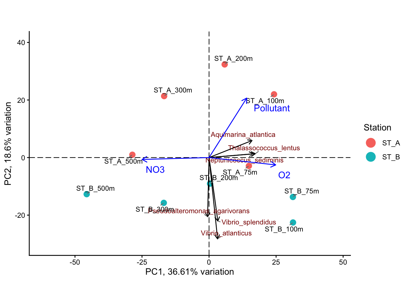
5.4.5 Example of interpretation
The PCA ordination reveals a clear structure in the dataset, with the first two axes explaining a substantial proportion of the total variance (PC1: 36.6%, PC2: 18.6%). This indicates that the main patterns of variation in community composition are well captured in this two-dimensional representation. The distribution of samples along PC1 suggests the presence of a strong underlying gradient structuring the data.
Identification of the main environmental gradient (PC1) : Depth
The main gradient observed along PC1 is strongly associated with opposing patterns of oxygen (O2) and nitrate (NO3), as shown by the direction of the environmental vectors. These variables are negatively correlated and represent opposite ends of the same environmental gradient. This pattern is consistent with a depth-related gradient in marine environments, where oxygen concentrations decrease and nutrient concentrations increase with depth due to biological and biogeochemical processes.
Secondary gradient (PC2) : Station
The second axis (PC2) captures a smaller proportion of the variance (18.6%) and appears to reflect differences between sampling stations. The projection of the pollutant variable along this axis suggests that this gradient may be linked to station-specific environmental conditions, potentially reflecting localized or anthropogenic influences.
Variation in community composition along the gradients
The distribution of taxa along the PCA axes indicates a progressive turnover in community composition. Taxa associated with high oxygen (T. lentus, N. sediminis, A. atlantica) levels are linked to surface or well-oxygenated environments, while those aligned with nitrate (not shown in the figure) are associated with deeper or nutrient-rich conditions. Additionally, variation along PC2 suggests differences in community composition between stations (Vibrio spp.).
Contribution of environmental variables (envfit)
The envfit analysis confirms that O2 and NO3 are significant drivers (p < 0.05) of the primary gradient (PC1), while the pollutant variable is associated with the secondary gradient (PC2, p <0.05). In contrast, other variables such as NH4, salinity, pH, and turbidity show weaker or non-significant relationships with the ordination.
Interpretation and limitations
Overall, this analysis highlights a dominant depth-related environmental gradient structuring microbial communities, along which oxygen decreases and nutrients increase. A secondary gradient, likely related to station-specific conditions, also contributes to the observed structure. However, it is important to note that this approach identifies correlations rather than causal relationships, as environmental variables are fitted a posteriori onto the PCA.
This exploratory strategy (PCA is descriptive) therefore provides valuable insights into potential drivers of community variation, but does not formally quantify the contribution of environmental variables. To address this limitation, a constrained ordination method such as RDA can be applied to directly model and quantify the fraction of biological variation (i.e. the variance) explained by environmental factors.
6. Testing the effect of environmental and categorical variables (PERMANOVA)
IMPORTANT : envfit identifies variables correlated with PCA axes (PC1 and PC2 ->56% of total variance ), but remains exploratory. PERMANOVA, in contrast, tests the effect of variables on the full data matrix, providing a formal statistical validation of the observed patterns.
6.1 Effect of sampling station & Depth on community composition
Following the exploratory PCA and envfit analyses, which revealed a clear structure in the data and suggested potential environmental drivers, it is necessary to formally test whether the observed patterns are statistically significant. In particular, the visual separation of samples (PC1 and PC2) according to sampling stations and Depth needs to be validated.
PERMANOVA (Permutational Multivariate Analysis of Variance) provides a non-parametric framework to test for differences in community composition between predefined groups. Unlike PCA, which is purely descriptive, PERMANOVA allows the assessment of whether the centroids of groups differ significantly in multivariate space, based on the original data matrix.This approach therefore complements the PCA by moving from visual interpretation to statistical testing, enabling the validation of group effects such as station or other categorical variables. Importantly, PERMANOVA relies on permutation tests and does not assume normality, making it well suited for ecological and compositional data.
However, it is also necessary to verify that any significant result is not driven by differences in dispersion among groups. This will be assessed using a test of homogeneity of multivariate dispersion (betadisper), ensuring that detected differences reflect true shifts in community composition rather than variability within groups.
Remember :
envfit → correlation against PCA1/PCA2 (a part of the whole)
PERMANOVA → Global effect on the whole community structure
The idea : PERMANOVA statistically confirms the effect suggested by envfit
6.1.1 Data preparation
# Use the same matrix as for PCA:
# otu_table with samples in rows, taxa in columns
Perm_data <- t(as.matrix(physeq_clr@otu_table))

# Extract metadata
meta <- data.frame(sample_data(physeq_clr))

# Make sure grouping variables are factors -> groups
meta$Station <- as.factor(meta$Station)
meta$Depth_cat <- as.factor(meta$Depth_cat)
6.1.2 Permanova test on physeq_clr_dist (already calculated)
6.1.2.1 Effect of sampling station on community composition (PERMANOVA)
set.seed(123)

permanova_station <- vegan::adonis2(
  physeq_clr_dist ~ Station,
  data = meta,
  permutations = 999
)

permanova_station
Permutation test for adonis under reduced model
Permutation: free
Number of permutations: 999
vegan::adonis2(formula = physeq_clr_dist ~ Station, data = meta, permutations = 999)
Df SumOfSqs R2 F Pr(>F)
Model 1 2540 0.148 1.39 0.17
Residual 8 14573 0.852
Total 9 17113 1.000 Although some separation between stations was observed in the PCA, PERMANOVA did not detect a significant effect, indicating that this pattern does not reflect a strong or consistent difference in community composition.
Why do not use betadispersion test (betadisper) ?
6.1.2.2 Effect of Depth category on community composition (PERMANOVA)
set.seed(123)

permanova_station <- vegan::adonis2(
  physeq_clr_dist ~ Depth_cat,
  data = meta,
  permutations = 999
)

permanova_station
Permutation test for adonis under reduced model
Permutation: free
Number of permutations: 999
vegan::adonis2(formula = physeq_clr_dist ~ Depth_cat, data = meta, permutations = 999)
Df SumOfSqs R2 F Pr(>F)
Model 2 7113 0.416 2.49 0.004 **
Residual 7 10000 0.584
Total 9 17113 1.000
---
Signif. codes: 0 '***' 0.001 '**' 0.01 '*' 0.05 '.' 0.1 ' ' 1Check the dispersion within groups
# Test homogeneity of multivariate dispersion among depth categories
bd_depth <- vegan::betadisper(physeq_clr_dist, meta$Depth_cat)

# Permutation test
vegan::permutest(bd_depth, permutations = 999)
Permutation test for homogeneity of multivariate dispersions
Permutation: free
Number of permutations: 999

Response: Distances
          Df Sum Sq Mean Sq    F N.Perm Pr(>F)
Groups     2   93.1    46.5 2.44    999   0.17
Residuals  7  133.7    19.1
Conclusion
No significant differences in dispersion were detected among depth categories (p = 0.171), indicating that group variances are homogeneous. This supports the validity of the PERMANOVA results.
The significant effect of depth category (p = 0.004) indicates that community composition differs across depth ranges, supporting the presence of a structured ecological gradient. This result is consistent with the PCA, where depth-related environmental variables were identified as major drivers of community variation.
6.1.2.3 PERMANOVA analysis of the combined effects of depth and station
In a combined model, each variable is tested for its UNIQUE contribution. If two variables are correlated, one may lose significance because it does not explain additional variation beyond the other. Therefore, only variables that explain a unique portion of the variation remain significant. This allows the identification of the main drivers of community structure while avoiding redundancy between explanatory variables.
Test looking for :
Depth → the unique contribution of depth after accounting for station
Station → the unique contribution of Station after accounting for depth
set.seed(123)

permanova_combined <- vegan::adonis2(
  physeq_clr_dist ~ Depth_cat + Station,
  data = meta,
  permutations = 999,
  by = "margin" # Test the independent (marginal) effect of each variable in the model
)

permanova_combined
Permutation test for adonis under reduced model
Marginal effects of terms
Permutation: free
Number of permutations: 999
vegan::adonis2(formula = physeq_clr_dist ~ Depth_cat + Station, data = meta, permutations = 999, by = "margin")
Df SumOfSqs R2 F Pr(>F)
Depth_cat 2 7113 0.416 2.86 0.001 ***
Station 1 2540 0.148 2.04 0.049 *
Residual 6 7459 0.436
Total 9 17113 1.000
---
Signif. codes: 0 '***' 0.001 '**' 0.01 '*' 0.05 '.' 0.1 ' ' 1The combined model showed that depth has a strong and significant effect on community composition (p=0.001), confirming it as the main environmental driver of the observed patterns. Station also became significant when tested together with depth, indicating that it explains an additional part of the variation that is not related to depth.
Depth and station influence the community structure in different ways. While depth represents a major environmental gradient, station reflects a secondary effect, possibly linked to local conditions or other unmeasured factors. Testing both variables together allows us to distinguish their unique contributions.
The MOST IMPORTANT : When station was tested alone, its effect was not significant because it was masked by the stronger effect of depth. In other words, most of the variation in the data is driven by depth, making it difficult to detect the smaller contribution of station. Removing the effect of depth, the remaining variation reveals the weaker but real effect of station.
6.2 Effect of environmental variables on community composition (PERMANOVA)
PCA and envfit identified environmental variables associated with the main gradients of the data. PERMANOVA was used to formally test the effect of environmental variables on community composition.
Collinearity (= variables that describe the same thing, correlated) between environmental variables can lead to unstable results, as shared variation reduces the unique contribution of each variable. Therefore, only non-redundant variables should be included in the analysis.
Rules : 1 gradient = 1 variable
Are No3 and O2 are collinears?
Envfit results is a good approach to select which variable to use
Depth, oxygen, and nitrate describe the same underlying environmental gradient and are therefore highly correlated. To avoid redundancy, only one representative variable was included in the PERMANOVA model.
Is community structure driven by depth (physical gradient)?
Is it influenced by oxygen availability (physiological constraint)?
Or by nitrate concentration (nutrient availability)?
These variables describe the same gradient but address different ecological questions. The choice of selected environmental variable depends on the ecological question addressed. SO YOU & your project!!! But you can additionally use correlation testing for helping the decision.
6.2.1 Collinearity check : correlation matrix
#spearman correlation -> non parametric
cor_mat <- stats::cor(env_sub, method = "spearman")

# Visualization
corrplot::corrplot(cor_mat, method = "color", type = "upper",tl.cex = 0.7,addCoef.col = "black")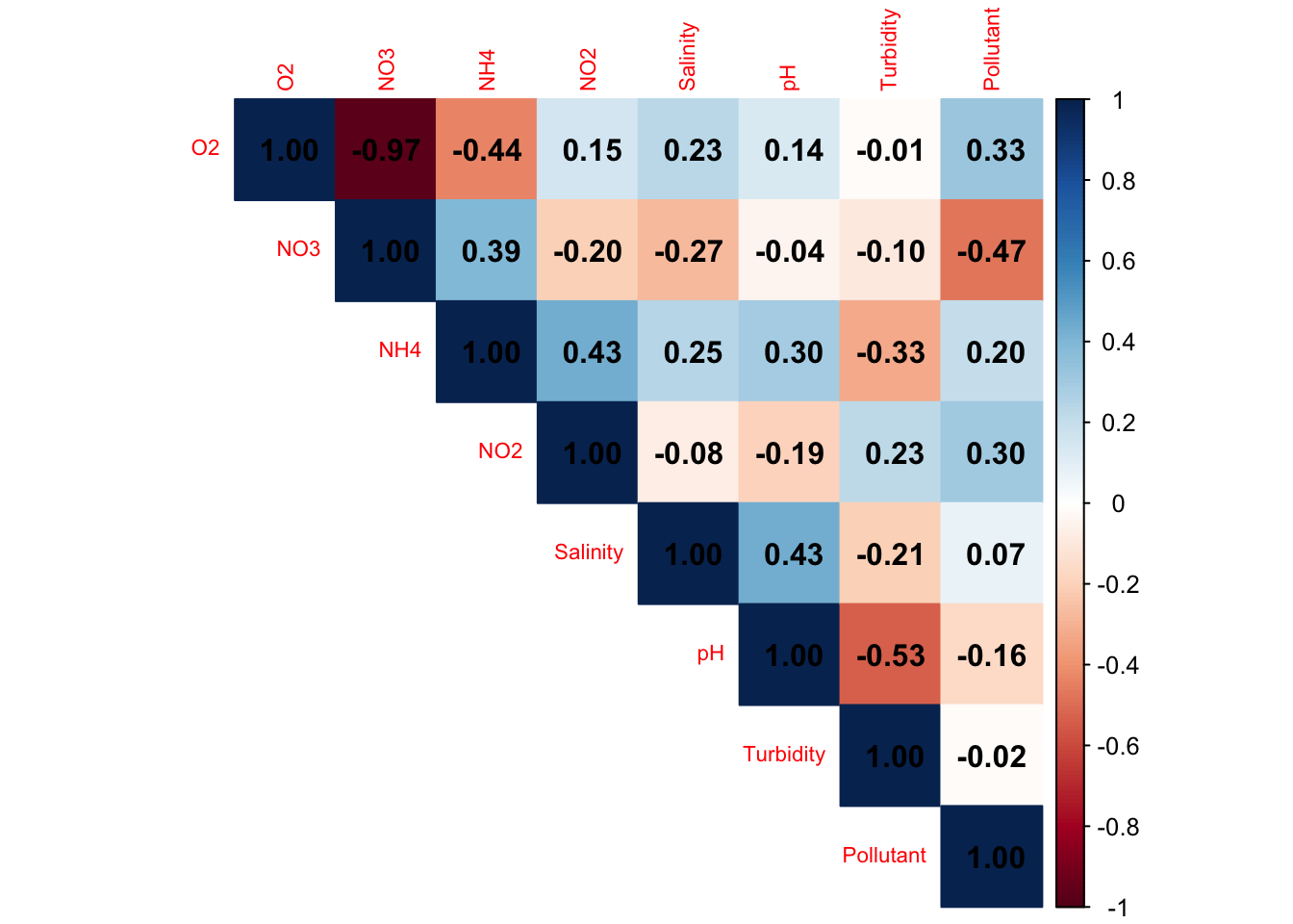
|r| > 0.7–0.8 → redundancy. Conclusion?
6.2.2 PERMANOVA analysis of the combined effects of O2 and Polluant
permanova_combined2 <- vegan::adonis2(
  physeq_clr_dist ~ O2 + Pollutant,
  data = meta,
  permutations = 999,
  by = "margin" # Test the independent (marginal) effect of each variable in the model
)

permanova_combined2
Permutation test for adonis under reduced model
Marginal effects of terms
Permutation: free
Number of permutations: 999
vegan::adonis2(formula = physeq_clr_dist ~ O2 + Pollutant, data = meta, permutations = 999, by = "margin")
Df SumOfSqs R2 F Pr(>F)
O2 1 4590 0.268 3.76 0.001 ***
Pollutant 1 2620 0.153 2.14 0.038 *
Residual 7 8551 0.500
Total 9 17113 1.000
---
Signif. codes: 0 '***' 0.001 '**' 0.01 '*' 0.05 '.' 0.1 ' ' 1Tests of multivariate dispersion (betadisper) were not performed for environmental variables, as these analyses require predefined groups and are not applicable to continuous predictors.
7. Constrained ordination: redundancy analysis (RDA) of environmental drivers of community composition
Unlike unconstrained ordination methods such as PCA, which explore, describe the main structure of a single dataset, direct gradient analyses explicitly incorporate environmental variables into the ordination process. PCA is therefore considered an exploratory and passive approach, where patterns are interpreted a posteriori. In contrast, RDA models community composition (response variables) as a function of environmental variables (explanatory variables).
MOST IMPORTANTLY : It allows the identification of the fraction of biological variation that can be explained by the selected environmental factors, while also enabling formal statistical testing of these relationships.
In this section, we apply RDA to investigate how selected environmental variables structure community composition. This approach builds on previous PCA, envfit, and PERMANOVA analyses by moving from exploratory patterns to a constrained and quantitative modeling of environmental effects.
Environmental variables were selected based on ecological relevance and envfit results, with collinearity assessed using correlation analysis. A parsimonious RDA model was then fitted and tested using permutation-based ANOVA.
A good approach is :
1. Pre-selection of variables based on envfit results and ecological relevance –> DONE
2. Removal of redundant variables using correlation analysis –> DONE
3. Optional stepwise selection (ordistep) to refine the model (replace 1 and 2)
4. Model validation using VIF and permutation tests in RDA
7.1 Data preparation : Otu_table matrix & environmental variables
# Standardize environmental variables (different units!!)
env_scaled <- as.data.frame(scale(env_sub))

# Extract the CLR-transformed community matrix from phyloseq
clr_table <- as.matrix(otu_table(physeq_clr))

# Ensure samples are rows and taxa are columns
if (taxa_are_rows(clr_table)) { clr_table <- t(clr_table)}
7.2 Run the model with the selected environmental variables
# Run the RDA with selected environmental variables
rda_selected <- vegan::rda(clr_table ~ O2 + Pollutant, data = env_scaled)
summary(rda_selected)
Call:
rda(formula = clr_table ~ O2 + Pollutant, data = env_scaled)
Partitioning of variance:
Inertia Proportion
Total 1901 1.0
Constrained 951 0.5
Unconstrained 950 0.5
Eigenvalues, and their contribution to the variance
Importance of components:
RDA1 RDA2 PC1 PC2 PC3 PC4
Eigenvalue 663.282 288.042 201.033 192.637 143.7010 122.9862
Proportion Explained 0.349 0.151 0.106 0.101 0.0756 0.0647
Cumulative Proportion 0.349 0.500 0.606 0.707 0.7829 0.8476
PC5 PC6 PC7
Eigenvalue 114.5186 92.7467 82.5303
Proportion Explained 0.0602 0.0488 0.0434
Cumulative Proportion 0.9078 0.9566 1.0000
Accumulated constrained eigenvalues
Importance of components:
RDA1 RDA2
Eigenvalue 663.282 288.042
Proportion Explained 0.697 0.303
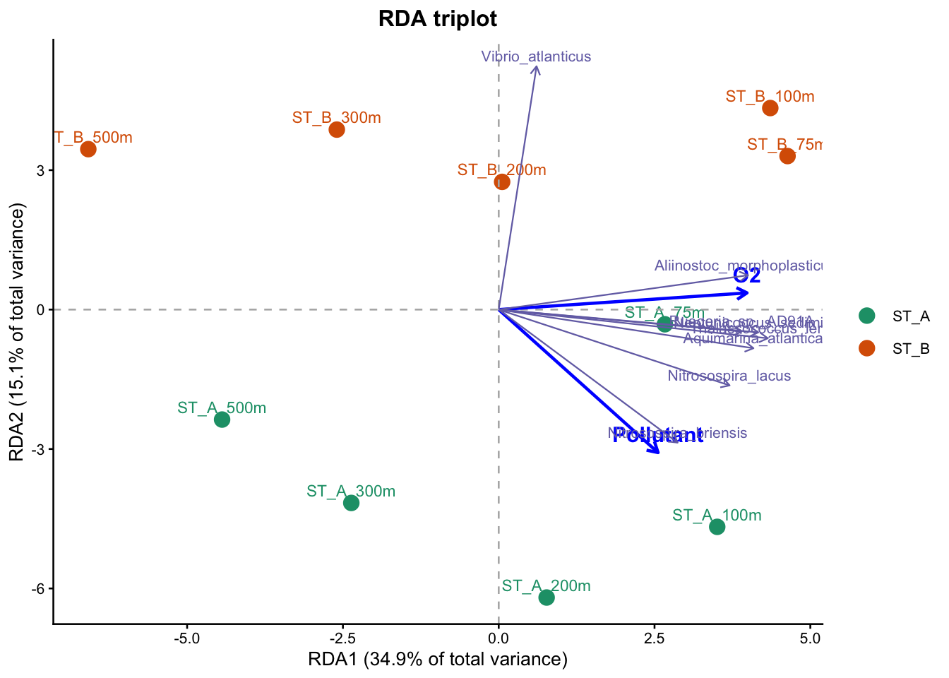
Cumulative Proportion 0.697 1.000The RDA model explained 50% of the total variation in community composition. The first constrained axis (RDA1) accounted for 69.7% of the explained variance (34.9% of total variance), representing the main environmental gradient. The second axis (RDA2) explained 30.3% of the constrained variance (15.1% of total variance), reflecting a secondary effect.
7.3 Assessment of multicollinearity using variance inflation factors (VIF)
Multicollinearity among environmental variables was assessed using variance inflation factors (VIF). VIF quantifies how much the variance of a variable is inflated due to its correlation with other variables in the model. High VIF values indicate redundancy between predictors. Values above 10 suggest potential collinearity issues and should be carefully examined.
Here, VIF was used to assess residual collinearity in the final RDA model.
# Check residual multicollinearity in the RDA model
vegan::vif.cca(rda_selected)
O2 Pollutant
1.475 1.475 Conclusion ?
7.4 Assessment of model performance (R² and adjusted R²)
The adjusted R² was used to account for the number of explanatory variables and avoid overestimating the model’s explanatory power.
# Unadjusted R^2 retrieved from the rda object
R2 <- vegan::RsquareAdj(rda_selected)$r.squared
R2
[1] 0.5003# Adjusted R^2 retrieved from the rda object
R2adj <- vegan::RsquareAdj(rda_selected)$adj.r.squared
R2adj[1] 0.3575The RDA model explained 50% of the total variation in community composition. However, after adjusting for model complexity, the explained variance decreased to 35%, indicating that part of the initial explanatory power was due to the number of variables included. The adjusted R² therefore provides a more conservative and reliable estimate of the model’s performance.
Therefore, what were the approximate proportion explained for RDA1 and RDA2 of the Total variance ?
Remember : The adjusted R² is used to assess the explanatory power of the model, whereas the RDA plot is based on the raw RDA1 and RDA2 axes derived from the constrained ordination.
7.5 Variance partitioning of environmental variables in the RDA model
Variance partitioning is used to break down the adjusted explained variation into the unique contributions of each environmental variable and their shared effects. It helps to distinguish independent from overlapping influences on community compositio, allowing a more detailed interpretation of the final RDA model.
# Variance partitioning between O2 and Pollutant of the model
varpart_res <- vegan::varpart(
  clr_table, #matrix table
  ~ O2,
  ~ Pollutant,
  data = env_scaled
)

varpart_res
Partition of variance in RDA

Call: vegan::varpart(Y = clr_table, X = ~O2, ~Pollutant, data =
env_scaled)

Explanatory tables:
X1:  ~O2
X2:  ~Pollutant

No. of explanatory tables: 2
Total variation (SS): 17113
            Variance: 1901.5
No. of observations: 10

Partition table:
                     Df R.squared Adj.R.squared Testable
[a+c] = X1            1   0.34723       0.26563     TRUE
[b+c] = X2            1   0.23209       0.13610     TRUE
[a+b+c] = X1+X2       2   0.50031       0.35754     TRUE
Individual fractions
[a] = X1|X2           1                 0.22143     TRUE
[b] = X2|X1           1                 0.09191     TRUE
[c]                   0                 0.04420    FALSE
[d] = Residuals                         0.64246    FALSE
---
Use function 'rda' to test significance of fractions of interest
The model explained 50% of the total variation (35.7% after adjustment). O2 was the main contributor, explaining 22.1% independently, while Pollutant explained 9.2%. A small shared fraction (4.4%) indicated limited overlap between variables. The remaining 64.2% of the variation was not explained by the model.
Community composition is primarily structured by an oxygen-driven gradient, with an additional and largely independent contribution from pollutant. The limited shared variance suggests limited collinearity between and indicates that these factors act on distinct ecological dimensions.
fractions <- varpart_res$part$indfract

vals <- c(
  O2_unique = fractions["[a] = X1|X2", "Adj.R.squared"],
  Pollutant_unique = fractions["[b] = X2|X1", "Adj.R.squared"],
  Shared = fractions["[c]", "Adj.R.squared"],
  Residual = fractions["[d] = Residuals", "Adj.R.squared"]
)

vals
O2_unique Pollutant_unique Shared Residual
0.22143 0.09191 0.04420 0.64246 bp <- barplot(
vals,
col = c("#1b9e77", "#d95f02", "#7570b3", "grey70"),
ylab = "Adjusted proportion of variance",
main = "Variance partitioning",
las = 2
)
text(bp, vals, labels = round(vals, 2), pos = 3)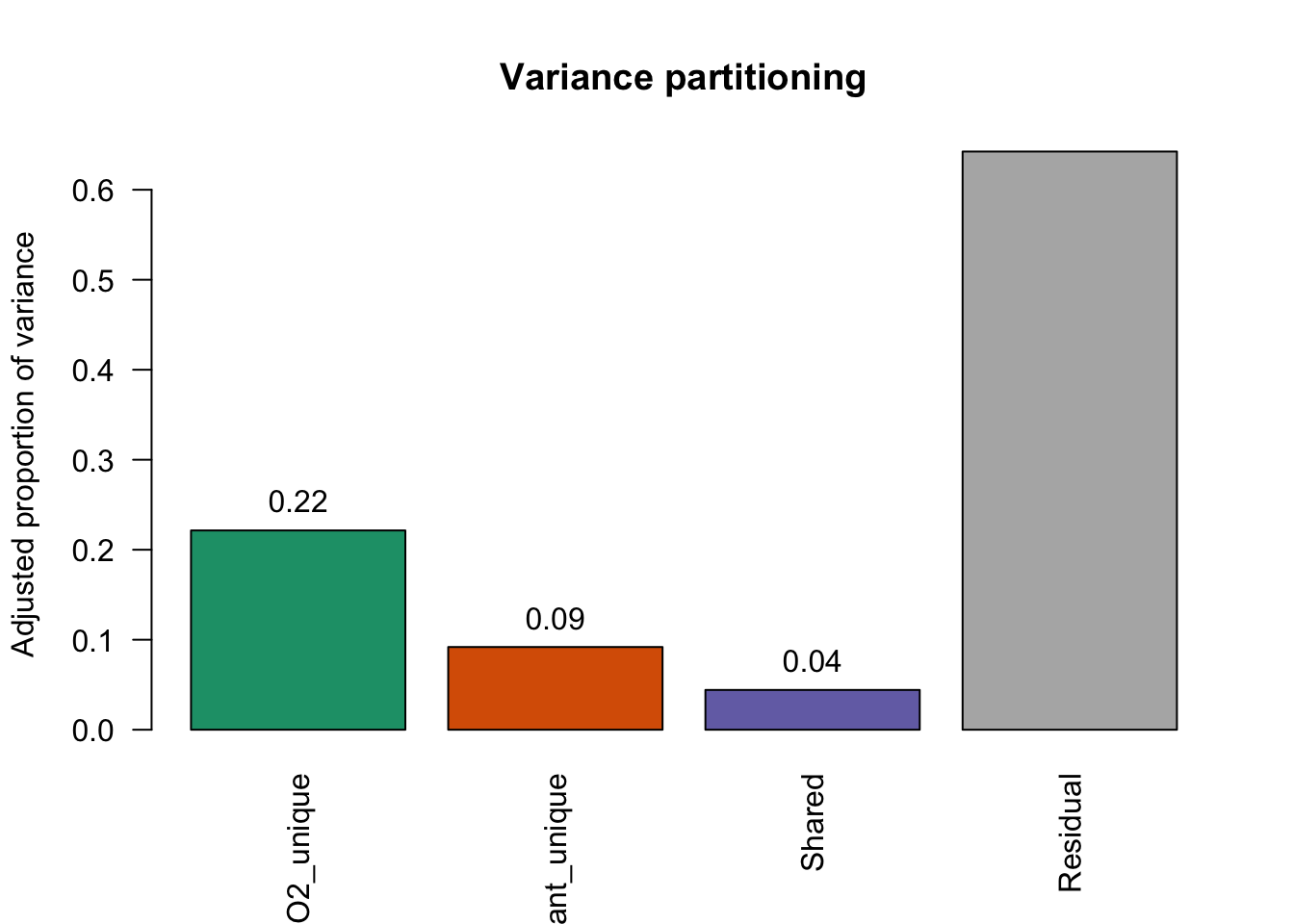
Although variance partitioning helps to disentangle the contributions of environmental variables, statistical testing is required to determine whether these effects are significant. To this end, permutation-based ANOVA tests were applied to the RDA model, its variables, and its axes.
7.6 Significance testing of the RDA model, variables, and axes
After fitting the RDA model (Section 7.2), significance tests were conducted to determine whether the relationships observed in the ordination are statistically supported.
Specifically, three tests were conducted:
a global test to assess the significance of the overall RDA model
a test of individual environmental variables to identify significant predictors
a test of constrained axes to evaluate their contribution to the model (true ecological gradient?)
7.6.1 Global test
# Test overall significance of the RDA model
anova(rda_selected, permutations = 999)
Permutation test for rda under reduced model
Permutation: free
Number of permutations: 999
Model: rda(formula = clr_table ~ O2 + Pollutant, data = env_scaled)
Df Variance F Pr(>F)
Model 2 951 3.5 0.001 ***
Residual 7 950
---
Signif. codes: 0 '***' 0.001 '**' 0.01 '*' 0.05 '.' 0.1 ' ' 17.6.2 Individual environmental variables
# Test significance of each environmental variable
anova(rda_selected, by = "term", permutations = 999)
Permutation test for rda under reduced model
Terms added sequentially (first to last)
Permutation: free
Number of permutations: 999
Model: rda(formula = clr_table ~ O2 + Pollutant, data = env_scaled)
Df Variance F Pr(>F)
O2 1 660 4.86 0.001 ***
Pollutant 1 291 2.14 0.037 *
Residual 7 950
---
Signif. codes: 0 '***' 0.001 '**' 0.01 '*' 0.05 '.' 0.1 ' ' 17.6.3 Constrained axes
# Test significance of each constrained axis
anova(rda_selected, by = "axis", permutations = 999)
Permutation test for rda under reduced model
Forward tests for axes
Permutation: free
Number of permutations: 999
Model: rda(formula = clr_table ~ O2 + Pollutant, data = env_scaled)
Df Variance F Pr(>F)
RDA1 1 663 4.89 0.001 ***
RDA2 1 288 2.43 0.002 **
Residual 7 950
---
Signif. codes: 0 '***' 0.001 '**' 0.01 '*' 0.05 '.' 0.1 ' ' 17.6.4 Coordinates of environmental variables
vegan::scores(rda_selected, display = "bp") RDA1 RDA2
O2 0.9959 0.08991
Pollutant 0.6391 -0.76910
attr(,"const")
[1] 11.44The RDA model was significant and explained 50% of the total variation in community composition. After accounting for model complexity, the adjusted R² indicated that 35% of the variation is reliably explained by the selected environmental variables.
Oxygen was identified as the main explanatory variable (RDA1), accounting for a substantial part of the variation, while pollutant also contributed significantly, representing a secondary but meaningful effect (RDA2). These results indicate that community composition is strongly structured along an oxygen-related gradient, with an additional contribution from pollutant, and that these effects are statistically supported by the RDA model.
7.7 Don’t hate me : the famous Optional stepwise selection (ordistep) to refine the model (7.)
To complement the previous variable selection based on ecological reasoning and correlation analysis, a stepwise selection procedure (ordistep) was applied as an independent and quantitative approach to confirm the relevance of the selected variables.
A forward stepwise selection (ordistep) was performed, starting from a null model and progressively adding variables that significantly improve the RDA model based on permutation tests.
# Run the RDA with ALL(~ .) environmental variables
rda_full <- vegan::rda(clr_table ~ ., data = env_scaled)

# Build the null model with no explanatory variable (~ 1)
rda_null <- vegan::rda(clr_table ~ 1, data = env_scaled)

# Use stepwise selection to identify the most relevant variables
set.seed(123)
rda_step <- vegan::ordistep(
  object = rda_null,                 # starting point: null model
  scope = formula(rda_full),         # candidate variables to test
  direction = "forward",             # add variables step by step
  permutations = how(nperm = 999),   # permutation test for significance
  trace = TRUE                       # print model selection progress
)
Start: clr_table ~ 1

            Df  AIC    F Pr(>F)
+ O2         1 74.2 4.26  0.001 ***
+ NO3        1 74.2 4.22  0.001 ***
+ Pollutant  1 75.8 2.42  0.016 *
+ NH4        1 76.9 1.37  0.176
+ NO2        1 77.3 1.02  0.396
+ Turbidity  1 77.7 0.62  0.854
+ Salinity   1 77.7 0.62  0.857
+ pH         1 77.7 0.60  0.890
---
Signif. codes:  0 '***' 0.001 '**' 0.01 '*' 0.05 '.' 0.1 ' ' 1

Step: clr_table ~ O2

            Df  AIC    F Pr(>F)
+ Pollutant  1 73.5 2.14  0.035 *
+ NH4        1 73.8 1.89  0.067 .
+ NO3        1 74.0 1.72  0.076 .
+ NO2        1 74.7 1.15  0.297
+ Turbidity  1 75.0 0.86  0.533
+ Salinity   1 75.2 0.76  0.655
+ pH         1 75.2 0.75  0.664
---
Signif. codes:  0 '***' 0.001 '**' 0.01 '*' 0.05 '.' 0.1 ' ' 1

Step: clr_table ~ O2 + Pollutant

            Df  AIC    F Pr(>F)
+ NH4        1 73.4 1.44   0.18
+ NO3        1 73.6 1.28   0.21
+ NO2        1 73.8 1.10   0.33
+ Turbidity  1 73.9 1.04   0.37
+ pH         1 74.1 0.90   0.53
+ Salinity 1 74.2 0.86 0.53summary(rda_step)
Call:
rda(formula = clr_table ~ O2 + Pollutant, data = env_scaled)

Partitioning of variance:
              Inertia Proportion
Total            1901        1.0
Constrained       951        0.5
Unconstrained     950        0.5

Eigenvalues, and their contribution to the variance

Importance of components:
                         RDA1    RDA2     PC1     PC2      PC3      PC4
Eigenvalue            663.282 288.042 201.033 192.637 143.7010 122.9862
Proportion Explained    0.349   0.151   0.106   0.101   0.0756   0.0647
Cumulative Proportion   0.349   0.500   0.606   0.707   0.7829   0.8476
                           PC5     PC6     PC7
Eigenvalue            114.5186 92.7467 82.5303
Proportion Explained    0.0602  0.0488  0.0434
Cumulative Proportion   0.9078  0.9566  1.0000

Accumulated constrained eigenvalues
Importance of components:
                         RDA1    RDA2
Eigenvalue            663.282 288.042
Proportion Explained    0.697   0.303
Cumulative Proportion   0.697   1.000
Conclusion :)
7.8 RDA triplot of community composition and environmental variables
# =========================================================
# FINAL RDA TRIPLOT
# - samples colored by Station
# - sample labels = meta$Name
# - environmental vectors
# - top species with taxonomic labels from make_tax_labels()
# - axis labels = % of TOTAL variance
# =========================================================


# ---------------------------------------------------------
# 1. Sample scores
# ---------------------------------------------------------
sites <- as.data.frame(scores(rda_selected, display = "sites", scaling = 2))
sites$Name <- meta$Name
sites$Station <- meta$Station

# ---------------------------------------------------------
# 2. Environmental vectors
# ---------------------------------------------------------
env_vec <- as.data.frame(scores(rda_selected, display = "bp", scaling = 2))
env_vec$Variable <- rownames(env_vec)

# ---------------------------------------------------------
# 3. Species scores
# ---------------------------------------------------------
sp <- as.data.frame(scores(rda_selected, display = "species", scaling = 2))

# attach labels to species scores
sp$Label <-  taxa_names(physeq_clr)

# keep the most important species (largest distance from origin)
sp$dist <- sqrt(sp$RDA1^2 + sp$RDA2^2)
sp_top <- sp[order(sp$dist, decreasing = TRUE), ][1:8, ]

# ---------------------------------------------------------
# 4. Axis labels = % of TOTAL variance
# ---------------------------------------------------------
eig_constrained <- rda_selected$CCA$eig
total_inertia <- rda_selected$tot.chi

axis1_total <- round(100 * eig_constrained[1] / total_inertia, 1)
axis2_total <- round(100 * eig_constrained[2] / total_inertia, 1)

# ---------------------------------------------------------
# 5. Rescale arrows for display
# ---------------------------------------------------------
env_mult <- 4
env_vec$RDA1 <- env_vec$RDA1 * env_mult
env_vec$RDA2 <- env_vec$RDA2 * env_mult

sp_mult <- 6
sp_top$RDA1 <- sp_top$RDA1 * sp_mult
sp_top$RDA2 <- sp_top$RDA2 * sp_mult

# ---------------------------------------------------------
# 6. Final triplot
# ---------------------------------------------------------
ggplot(sites, aes(x = RDA1, y = RDA2, color = Station)) +

  # samples
  geom_point(size = 3.5) +
  geom_text(aes(label = Name), vjust = -0.6, size = 3, show.legend = FALSE) +

  # origin lines
  geom_hline(yintercept = 0, linetype = 2, color = "grey70") +
  geom_vline(xintercept = 0, linetype = 2, color = "grey70") +

  # environmental vectors
  geom_segment(
    data = env_vec,
    aes(x = 0, y = 0, xend = RDA1, yend = RDA2),
    arrow = arrow(length = unit(0.22, "cm")),
    color = "blue",
    linewidth = 0.8,
    inherit.aes = FALSE
  ) +
  geom_text(
    data = env_vec,
    aes(x = RDA1, y = RDA2, label = Variable),
    color = "blue",
    fontface = "bold",
    vjust = -0.7,
    size = 4,
    inherit.aes = FALSE
  ) +

  # species vectors
  geom_segment(
    data = sp_top,
    aes(x = 0, y = 0, xend = RDA1, yend = RDA2),
    arrow = arrow(length = unit(0.18, "cm")),
    color = "#7570b3",
    linewidth = 0.4,
    inherit.aes = FALSE
  ) +
  geom_text(
    data = sp_top,
    aes(x = RDA1, y = RDA2, label = Label),
    color = "#7570b3",
    size = 2.8,
    vjust = -0.5,
   # hjust = - 1.5,
    inherit.aes = FALSE
  ) +

  # station colors
  scale_color_manual(values = c("ST_A" = "#1b9e77", "ST_B" = "#d95f02")) +

  # labels
  labs(
    title = "RDA triplot",
    x = paste0("RDA1 (", axis1_total, "% of total variance)"),
    y = paste0("RDA2 (", axis2_total, "% of total variance)")
  ) +

  # theme
  theme_classic(base_size = 10) +
  theme(
    plot.title = element_text(face = "bold", hjust = 0.5),
    legend.title = element_blank()
  )
8. Diffential abundance analysis (DAA)
The goal of differential abundance testing is to identify specific taxa associated with metadata variables of interest. This is a difficult task. It is also one of the more controversial areas in microbiome data analysis as illustrated in this preprint. This is related to concerns that normalization and testing approaches have generally failed to control false discovery rates. For more details see these papers here and here.
There are many tools to perform DAA. The most popular tools, without going into evaluating whether or not they perform well for this task, are:
-ALDEx2
-ANCOM-BC
-conrcob
-DESeq2
-edgeR
-LEFse
-limma voom
-LinDA
-MaAsLin2
-metagenomeSeq
-IndVal
-t-test
-Wilcoxon test
Nearing et al. (2022) compared all these listed methods across 38 different datasets and showed that ALDEx2 and ANCOM-BC produce the most consistent results across studies. Because different methods use different approaches (parametric vs non-parametric, different normalization techniques, assumptions etc.), results can differ between methods.Therefore, it is highly recommended to pick several methods to get an idea about how robust and potentially reproducible your findings are depending on the method. Here, we will apply 3 methods that are currently used in microbial ecology or that can be recommended based on recent literature (ANCOM-BC, ALDEx2 and LEFse) and we will compare the results between them. For this, we will use the recent microbiome_marker package.
8.1 Linear discriminant analysis Effect Size (LEFse)
LEFSE has been developped by Segata et al. (2011). LEFse first use the non-parametric factorial Kruskal-Wallis (KW) sum-rank test to detect features with significant differential abundance with respect to the class of interest; biological consistency is subsequently investigated using a set of pairwise tests among subclasses using the (unpaired) Wilcoxon rank-sum test. As a last step, LEfSe uses LDA to estimate the effect size of each differentially abundant features.
Lefse : A quel point un taxon différencie les groupes. LDA donne un score d’effet. plus le score est élevé, plus il discrimine les groupes. LDA = 2 : effet modéré, >=3 : effet fort.
tax <- as.data.frame(tax_table(physeq))
colnames(tax) <- c("Kingdom", "Phylum", "Class", "Order", "Family", "Genus", "Species")
tax_table(physeq) <- as.matrix(tax)

physeq_lefse <- phyloseq::filter_taxa(
  physeq,
  function(x) sum(x > 0) >=10,
  prune = TRUE
)set.seed(123)
#LEFSE
mm_lefse <- microbiomeMarker::run_lefse(physeq_lefse, norm = "CPM",
wilcoxon_cutoff = 0.05,
group = "Station",
taxa_rank = "Species",
kw_cutoff = 0.05,
multigrp_strat = TRUE,
lda_cutoff = 2)
mm_lefse_table <- data.frame(mm_lefse@marker_table)
mm_lefse_table feature enrich_group ef_lda pvalue
marker1 Marinoscillum pacificum ST_A 4.206 0.009023
marker2 Colwellia psychrerythraea ST_A 3.899 0.009023
marker3 Methylococcus capsulatus ST_A 3.858 0.028280
marker4 Sneathiella glossodoripedis ST_A 3.581 0.009023
marker5 Dulcicalothrix necridiiformans ST_B 4.649 0.028280
marker6 Aliterella antarctica ST_B 4.225 0.028280
marker7 alpha proteobacterium HIMB5 ST_B 3.888 0.028280
marker8 Candidatus Thioglobus singularis ST_B 3.823 0.009023
marker9 Candidatus Paracaedibacter acanthamoebae ST_B 3.652 0.028280
padj
marker1 0.009023
marker2 0.009023
marker3 0.028280
marker4 0.009023
marker5 0.028280
marker6 0.028280
marker7 0.028280
marker8 0.009023
marker9 0.028280p_LDAsc <- microbiomeMarker::plot_ef_bar(mm_lefse)
p_abd <- microbiomeMarker::plot_abundance(mm_lefse, group = "Station")
gridExtra::grid.arrange(p_LDAsc, p_abd, nrow = 1)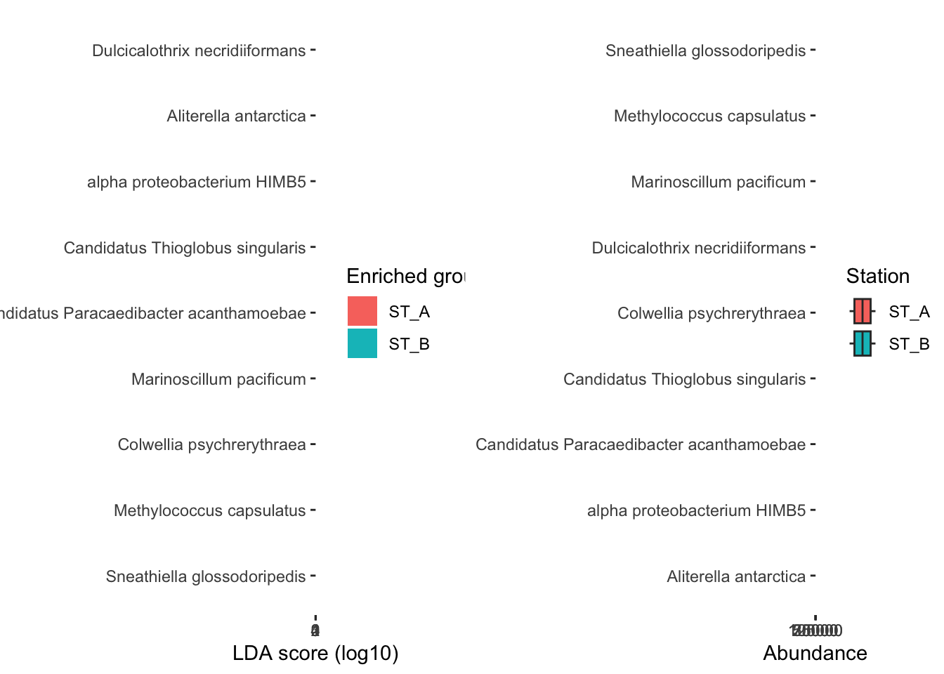
8.2 LDifferential analysis of compositions of microbiomes with bias correction (ANCOM-BC)
The ANCOM-BC methodology assumes that the observed sample is an unknown fraction of a unit volume of the ecosystem, and the sampling fraction varies from sample to sample. ANCOM-BC accounts for sampling fraction by introducing a sample-specific offset term in a linear regression framework, that is estimated from the observed data. The offset term serves as the bias correction, and the linear regression framework in log scale is analogous to log-ratio transformation to deal with the compositionality of microbiome data. Furthermore, this method provides p-values and confidence intervals for each taxon. It also controls the FDR and it is computationally simple to implement.
#ancomBC be careful you have to use the RAW data (physeq)!!!!!
mm_ancombc <- run_ancombc_patched(physeq, group = "Station",
                                            taxa_rank = "Species",
                                            pvalue_cutoff = 0.001,
                                            p_adjust = "fdr")

mm_ancombc_table <- data.frame(mm_ancombc@marker_table)
mm_ancombc_table
feature enrich_group ef_W
marker1 Marinoscillum pacificum ST_A -7.755
marker2 Pseudofulvibacter marinus ST_B 4.666
marker3 Weissella koreensis ST_A -4.404
marker4 Gemmatimonas aurantiaca ST_A -6.440
marker5 Roseisolibacter agri ST_A -4.389
marker6 endosymbiont of Acanthamoeba sp. UWC8 ST_A -4.801
marker7 Amylibacter marinus ST_B 6.572
marker8 Amylibacter ulvae ST_B 5.915
marker9 Litoreibacter albidus ST_A -4.248
marker10 Magnetospira sp. QH-2 ST_A -4.718
marker11 Magnetospira thiophila ST_A -5.554
marker12 Oceanibaculum nanhaiense ST_A -6.923
marker13 Oceanibaculum pacificum ST_A -4.176
marker14 Pelagibius litoralis ST_A -4.538
marker15 Candidatus Midichloria mitochondrii ST_A -4.318
marker16 Sneathiella chinensis ST_A -5.064
marker17 Sneathiella glossodoripedis ST_A -10.947
marker18 Erythrobacter sp. KY5 ST_A -4.471
marker19 Colwellia psychrerythraea ST_A -5.012
marker20 Sulfuriflexus mobilis ST_A -4.181
marker21 Methylococcus capsulatus ST_A -4.972
marker22 Oceanospirillum multiglobuliferum ST_A -4.418
marker23 Psychrobacter sp. AntiMn-1 ST_A -6.369
marker24 Vibrio atlanticus ST_B 11.857
marker25 Vibrio splendidus ST_B 7.200
pvalue
marker1 0.00000000000000880306620390830996250
marker2 0.00000307566004179538494481814005221
marker3 0.00001060774467484458856859474290557
marker4 0.00000000011963304056360941242400438
marker5 0.00001137411341978955302614833627883
marker6 0.00000158093836344779933136058414772
marker7 0.00000000004952377911133708658013857
marker8 0.00000000332128170293142930051073117
marker9 0.00002159748609148879385779759565445
marker10 0.00000238726158677344377001322203724
marker11 0.00000002786450368572924249543473134
marker12 0.00000000000442336069555603339583416
marker13 0.00002960307162162236405047316400996
marker14 0.00000567291761359228077581627613935
marker15 0.00001575046825106047766328239145839
marker16 0.00000040964517314504415370377075206
marker17 0.00000000000000000000000000068969067
marker18 0.00000777195940228717740267099650664
marker19 0.00000053734420269586082201450187579
marker20 0.00002904104123923733149297519984255
marker21 0.00000066132810971463706799705400616
marker22 0.00000994147363524016919702260691727
marker23 0.00000000019010475859647804131820754
marker24 0.00000000000000000000000000000001982
marker25 0.00000000000060404383669207901662650
padj
marker1 0.00000000000243258062767999619710
marker2 0.00015935763591552339047373310077
marker3 0.00043969101677230823521647096186
marker4 0.00000001416797008960459983075648
marker5 0.00044900666785740664258344545523
marker6 0.00009361413594987326837817964709
marker7 0.00000000684253548054974005372946
marker8 0.00000030592694797001723763235225
marker9 0.00077844852042800911657433049484
marker10 0.00013193599036234566969534587333
marker11 0.00000230996735554695433852915969
marker12 0.00000000073339320332319043283362
marker13 0.00098163785497299739513099581245
marker14 0.00027663815892164711268338961325
marker15 0.00059350628091496071894739294805
marker16 0.00003087234986702196246500379262
marker17 0.00000000000000000000000028587678
marker18 0.00035794190802755946820279397969
marker19 0.00003712152866957238586198900010
marker20 0.00098163785497299739513099581245
marker21 0.00004217238484257185428911648972
marker22 0.00043376219176916312909864092973
marker23 0.00000001969960560956003840807949
marker24 0.00000000000000000000000000001643
marker25 0.00000000012518808515443338838848an_ef <- microbiomeMarker::plot_ef_bar(mm_ancombc)
an_abd <- microbiomeMarker::plot_abundance(mm_ancombc, group = "Station")
gridExtra::grid.arrange(an_ef, an_abd, nrow = 1)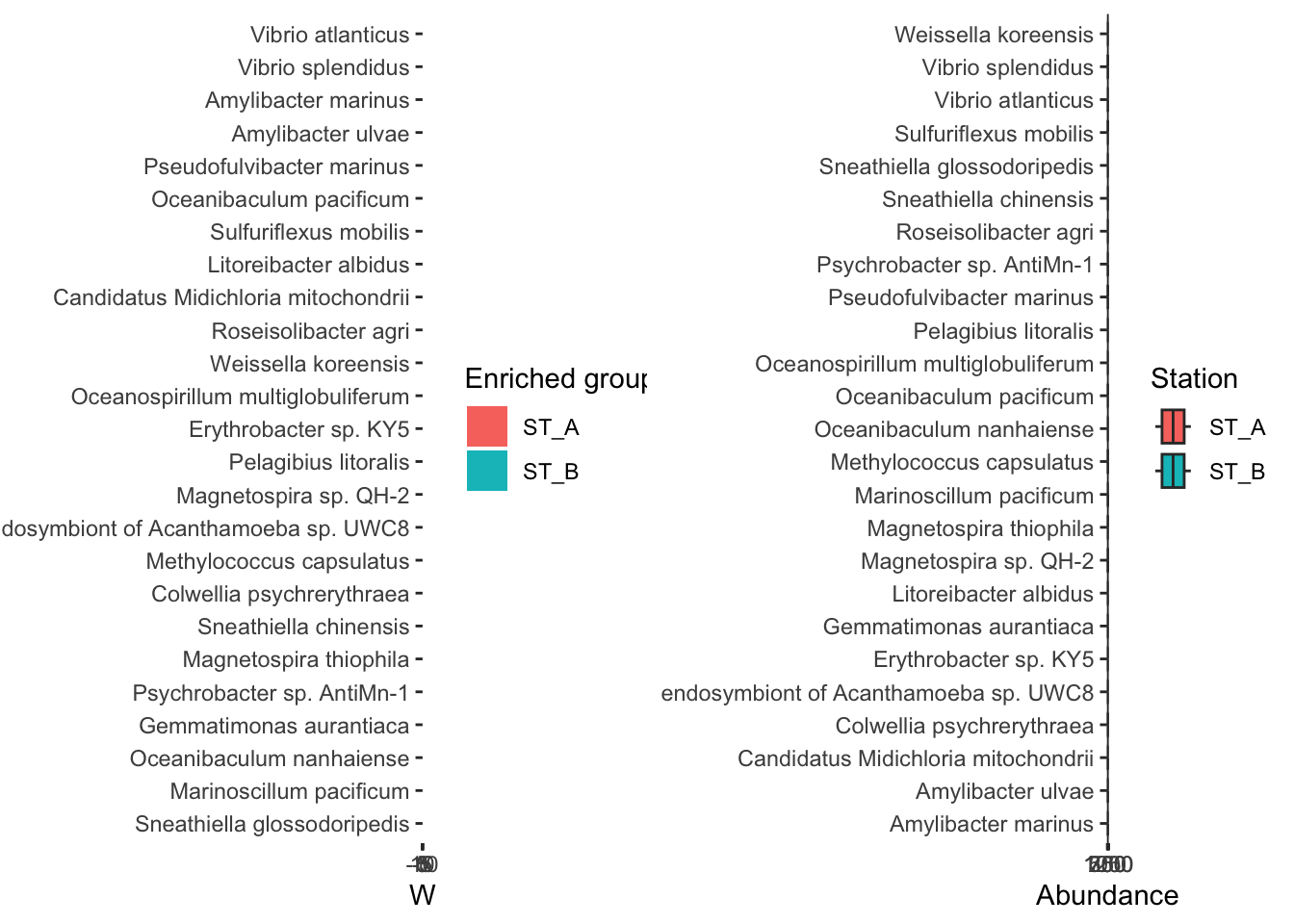
ANCOM-BC identifies 20 biomarkers. Are there all in common with the results of the LEFse analysis?