library(phyloseq)
library(ggplot2)
library(patchwork)
library(vegan)
library(permute)
library(plotly)
library(ComplexHeatmap)
library(grid)1 Prepare workspace
1.1 Load libraries
1.2 Load custom functions
devtools::load_all()1.3 Define output folder
output_alpha <- here::here("outputs", "alpha_diversity")
if (!dir.exists(output_alpha)) dir.create(output_alpha, recursive = TRUE)
1.4 Load the data and inspect the phyloseq object
Import the phyloseq object from …
physeq <- readRDS(here::here("data",
                             "asv_table",
                             "physeq.rds"))
2 Data Structure
2.1 Phyloseq object
physeqphyloseq-class experiment-level object
otu_table() OTU Table: [ 830 taxa and 10 samples ]
sample_data() Sample Data: [ 10 samples by 16 sample variables ]
tax_table() Taxonomy Table: [ 830 taxa by 7 taxonomic ranks ]
refseq() DNAStringSet: [ 830 reference sequences ]2.2 A Species table with the absolute counts
physeq@otu_table[1:10,1:10]OTU Table: [10 taxa and 10 samples]
taxa are rows
barcode13_combine_Q22 barcode14_combine_Q22 barcode17_combine_Q22
1002672 0 0 0
1002689 0 0 0
1002870 22 0 14
1006 154 26 23
1008307 24 0 0
1008392 48 17 0
102116 18 35 171
1026 110 0 64
1028 0 0 0
1031538 97 0 47
barcode18_combine_Q22 barcode19_combine_Q22 barcode20_combine_Q22
1002672 0 0 21
1002689 0 0 0
1002870 25 0 24
1006 51 0 45
1008307 0 0 0
1008392 0 0 16
102116 157 52 47
1026 127 37 41
1028 0 0 0
1031538 39 0 25
barcode21_combine_Q22 barcode22_combine_Q22 barcode23_combine_Q22
1002672 0 0 0
1002689 35 0 0
1002870 0 0 24
1006 28 16 166
1008307 20 0 0
1008392 38 0 18
102116 39 20 65
1026 0 61 144
1028 14 0 0
1031538 0 28 148
barcode24_combine_Q22
1002672 16
1002689 0
1002870 31
1006 335
1008307 0
1008392 31
102116 42
1026 311
1028 0
1031538 1852.3 A metadata table with information (e.g. physicochemical, categorical variables) about samples
physeq@sam_data SampleID Technology KIT Depth Station
barcode13_combine_Q22 barcode13_combine_Q22 Nanopore A 300m ST_A
barcode14_combine_Q22 barcode14_combine_Q22 Nanopore A 500m ST_A
barcode17_combine_Q22 barcode17_combine_Q22 Nanopore B 75m ST_B
barcode18_combine_Q22 barcode18_combine_Q22 Nanopore B 100m ST_B
barcode19_combine_Q22 barcode19_combine_Q22 Nanopore B 200m ST_B
barcode20_combine_Q22 barcode20_combine_Q22 Nanopore B 300m ST_B
barcode21_combine_Q22 barcode21_combine_Q22 Nanopore B 500m ST_B
barcode22_combine_Q22 barcode22_combine_Q22 Nanopore A 75m ST_A
barcode23_combine_Q22 barcode23_combine_Q22 Nanopore A 100m ST_A
barcode24_combine_Q22 barcode24_combine_Q22 Nanopore A 200m ST_A
Name Depths Depth_cat O2 NO3 NH4 NO2 Salinity
barcode13_combine_Q22 ST_A_300m 300 mid 128 18.5 0.94 0.11 38.32
barcode14_combine_Q22 ST_A_500m 500 deep 82 27.6 0.57 0.05 37.88
barcode17_combine_Q22 ST_B_75m 75 shallow 232 2.4 0.44 0.04 38.41
barcode18_combine_Q22 ST_B_100m 100 shallow 221 4.2 0.41 0.13 38.05
barcode19_combine_Q22 ST_B_200m 200 mid 171 10.8 0.52 0.17 37.72
barcode20_combine_Q22 ST_B_300m 300 mid 129 18.1 0.86 0.09 38.28
barcode21_combine_Q22 ST_B_500m 500 deep 82 28.5 0.43 0.03 37.95
barcode22_combine_Q22 ST_A_75m 75 shallow 228 2.0 0.40 0.06 38.10
barcode23_combine_Q22 ST_A_100m 100 shallow 208 4.8 0.69 0.11 37.83
barcode24_combine_Q22 ST_A_200m 200 mid 166 9.9 0.98 0.19 38.36
pH Turbidity Pollutant
barcode13_combine_Q22 8.06 1.8 9.44
barcode14_combine_Q22 7.98 2.1 9.33
barcode17_combine_Q22 8.12 1.5 9.30
barcode18_combine_Q22 8.03 2.3 9.30
barcode19_combine_Q22 7.95 1.9 9.00
barcode20_combine_Q22 8.10 2.0 8.84
barcode21_combine_Q22 8.01 1.7 8.57
barcode22_combine_Q22 7.92 2.2 9.74
barcode23_combine_Q22 8.08 1.6 9.83
barcode24_combine_Q22 8.00 1.8 9.662.4 A table of taxonomic classification level
physeq@tax_table[1:10,]Taxonomy Table: [10 taxa by 7 taxonomic ranks]:
kingdom phylum class order
1002672 "Bacteria" "Proteobacteria" "Alphaproteobacteria" "Pelagibacterales"
1002689 "Bacteria" "Acidobacteria" "Acidobacteriia" "Acidobacteriales"
1002870 "Bacteria" "Actinobacteria" "Rubrobacteria" "Gaiellales"
1006 "Bacteria" "Bacteroidetes" "Cytophagia" "Cytophagales"
1008307 "Bacteria" "Proteobacteria" "Gammaproteobacteria" "Cellvibrionales"
1008392 "Bacteria" "Fibrobacteres" "Chitinispirillia" "Chitinispirillales"
102116 "Bacteria" "Cyanobacteria" NA "Pleurocapsales"
1026 "Bacteria" "Bacteroidetes" "Cytophagia" "Cytophagales"
1028 "Bacteria" "Bacteroidetes" "Cytophagia" "Cytophagales"
1031538 "Bacteria" "Proteobacteria" "Gammaproteobacteria" "Oceanospirillales"
family genus
1002672 "Pelagibacteraceae" "Candidatus Pelagibacter"
1002689 "Acidobacteriaceae" "Occallatibacter"
1002870 "Gaiellaceae" "Gaiella"
1006 "Marivirgaceae" "Marivirga"
1008307 "Cellvibrionaceae" "Maricurvus"
1008392 "Chitinispirillaceae" "Chitinispirillum"
102116 "Dermocarpellaceae" "Stanieria"
1026 "Reichenbachiellaceae" "Marinoscillum"
1028 "Marivirgaceae" "Marivirga"
1031538 "Oceanospirillaceae" "Neptunomonas"
species
1002672 "Candidatus Pelagibacter sp. IMCC9063"
1002689 "Occallatibacter riparius"
1002870 "Gaiella occulta"
1006 "Marivirga tractuosa"
1008307 "Maricurvus nonylphenolicus"
1008392 "Chitinispirillum alkaliphilum"
102116 "Stanieria cyanosphaera"
1026 "Marinoscillum furvescens"
1028 "Marivirga sericea"
1031538 "Neptunomonas concharum" 2.5 A Phylogenetic tree (Need For Unifrac distance, See ANF2025)
https://anf-metabiodiv.github.io/course-material/practicals/beta_diversity.html
You have to use phy_tree for Unifrac distance.
bad_taxa <- c("mapped_unclassified", "unmapped")

# Remove unwanted artificial taxa (e.g., unmapped or unclassified reads)
# and keep only valid taxa for downstream phylogenetic analysis
physeq_tree <- phyloseq::prune_taxa(!phyloseq::taxa_names(physeq) %in% bad_taxa, physeq)
# Extract reference sequences
seqs <- phyloseq::refseq(physeq_tree)
# Perform multiple sequence alignment
alignment <- DECIPHER::AlignSeqs(seqs, anchor = NA)Determining distance matrix based on shared 9-mers:
================================================================================
Time difference of 22.1 secs
Clustering into groups by similarity:
================================================================================
Time difference of 0.2 secs
Aligning Sequences:
================================================================================
Time difference of 28.86 secs
Iteration 1 of 2:
Determining distance matrix based on alignment:
================================================================================
Time difference of 1.43 secs
Reclustering into groups by similarity:
================================================================================
Time difference of 0.06 secs
Realigning Sequences:
================================================================================
Time difference of 18.7 secs
Iteration 2 of 2:
Determining distance matrix based on alignment:
================================================================================
Time difference of 1.4 secs
Reclustering into groups by similarity:
================================================================================
Time difference of 0.06 secs
Realigning Sequences:
================================================================================
Time difference of 6.84 secs
Refining the alignment:
================================================================================
Time difference of 0.31 secs# Convert alignment to phyDat format
phang.align <- phangorn::phyDat(as(alignment, "matrix"), type = "DNA")
# Compute pairwise distances
dm <- phangorn::dist.ml(phang.align)
# Build Neighbor-Joining tree
treeNJ <- phangorn::NJ(dm)
# Root the tree using midpoint rooting
treeNJ_rooted <- phangorn::midpoint(treeNJ)
# Add the rooted tree to the filtered phyloseq object
phy_tree(physeq_tree) <- treeNJ_rooted#See phylogenetic tree included
physeq_treephyloseq-class experiment-level object
otu_table() OTU Table: [ 828 taxa and 10 samples ]
sample_data() Sample Data: [ 10 samples by 16 sample variables ]
tax_table() Taxonomy Table: [ 828 taxa by 7 taxonomic ranks ]
phy_tree() Phylogenetic Tree: [ 828 tips and 827 internal nodes ]
refseq() DNAStringSet: [ 828 reference sequences ]2.6 A table with the species sequences
Note: these are reference sequences from the query database.
physeq@refseqDNAStringSet object of length 830:
width seq names
[1] 1495 CCTTAGAAAGGAGGTAATCCAG...TGATCAAACTCTCAAGTTTAAT 1002672
[2] 1463 AGAGTTTGATCCTGGCTCAGAA...GTGAAGTCGTAACAAGGTAACC 1002689
[3] 1544 TGAGTTTGATCCTGGCTCAGGA...CGGCTGGATCACCTCCTTTCTA 1002870
[4] 1476 GATGAACGCTAGCGGCAGGCCT...AGGTAGCCGTACCGGAAGGTGT 1006
[5] 1500 GAGTTTGATCCTGGCTCAGATT...GTGAAGTCGTAACAAGGTAGCC 1008307
... ... ...
[826] 1493 AAAACGGAGAGTTTGATCCTGG...TGTGGCTGGATCACCTCCTTTT 99598
[827] 1393 GGGGTAACATTGTAGCTTGCTA...GAGCCGCCTAGGGTAAAACTGG 996801
[828] 1438 TCAGGATGAACGCTAGCGGCAG...ACAGGTAATTGGGGCTAAGTCG 998844
[829] 1488 NNNNNNNNNNNNNNNNNNNNNN...NNNNNNNNNNNNNNNNNNNNNN mapped_unclassified
[830] 1488 NNNNNNNNNNNNNNNNNNNNNN...NNNNNNNNNNNNNNNNNNNNNN unmapped3 Subsampling normalization
3.1 Rarefaction Curves
Before normalization by sub-sampling, let’s have a look at rarefaction curves, evaluate your sequencing effort and make decisions
3.1.1 Identify your minimum sample size
phyloseq::sample_sums(physeq)barcode13_combine_Q22 barcode14_combine_Q22 barcode17_combine_Q22
112842 39366 34688
barcode18_combine_Q22 barcode19_combine_Q22 barcode20_combine_Q22
64005 17012 49906
barcode21_combine_Q22 barcode22_combine_Q22 barcode23_combine_Q22
92390 10273 70829
barcode24_combine_Q22
94532 What is the minimum sample size?
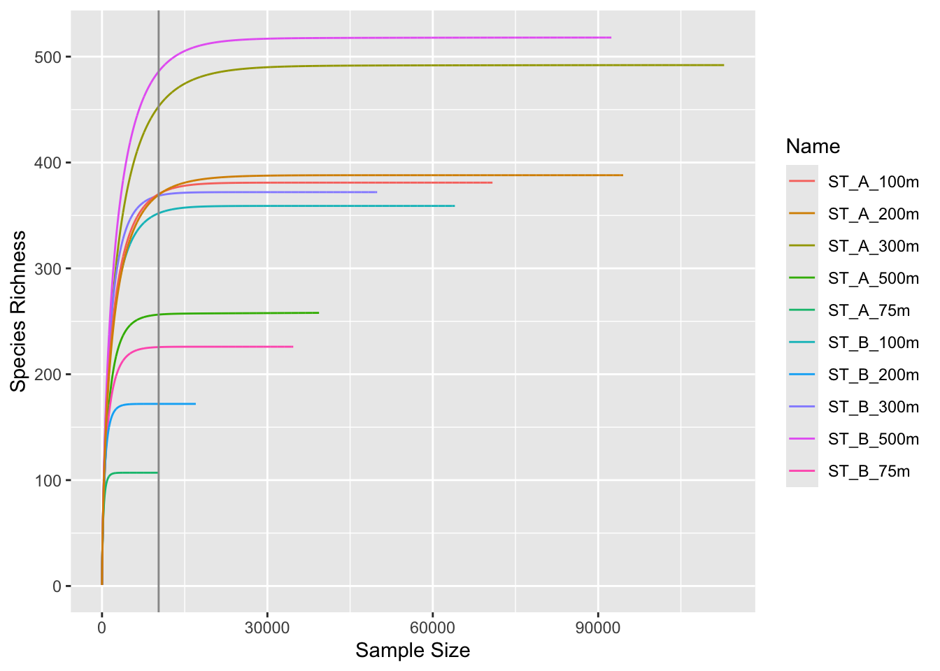
3.1.2 Run rarefaction curves using our custom function ggrare() (defined in R/alpha_diversity.R)
#Make rarefaction curves & Add min sample size line
ggrare(physeq, step = 10, color = "Name", se = FALSE) +
  geom_vline(xintercept = min(sample_sums(physeq)), color = "gray60")
rarefying sample barcode13_combine_Q22rarefying sample barcode14_combine_Q22
rarefying sample barcode17_combine_Q22rarefying sample barcode18_combine_Q22rarefying sample barcode19_combine_Q22rarefying sample barcode20_combine_Q22rarefying sample barcode21_combine_Q22rarefying sample barcode22_combine_Q22rarefying sample barcode23_combine_Q22rarefying sample barcode24_combine_Q22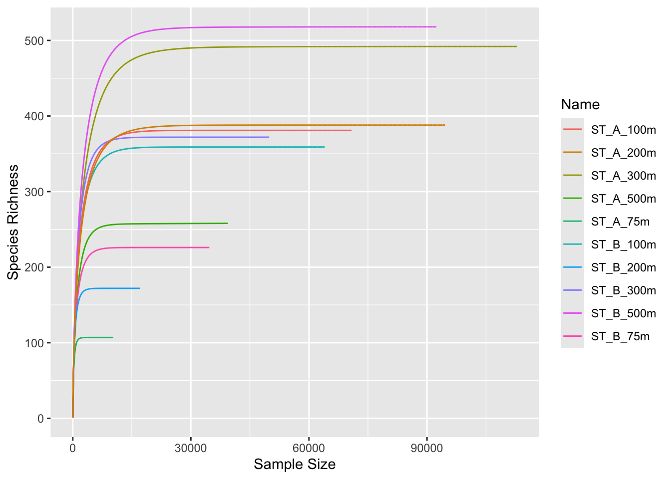
3.2 Normalization process for alpha diversity: sub-sampling
physeq_rar <- phyloseq::rarefy_even_depth(physeq, rngseed = TRUE)`set.seed(TRUE)` was used to initialize repeatable random subsampling.Please record this for your records so others can reproduce.Try `set.seed(TRUE); .Random.seed` for the full vector...28OTUs were removed because they are no longer
present in any sample after random subsampling...Check the number of sequences for each sample using sample_sums function
Did you lost a lot of species?
3.3 Run rarefaction curves on normalized data
p0 <- ggrare(physeq_rar, step = 10, color = "Name", se = TRUE)rarefying sample barcode13_combine_Q22
rarefying sample barcode14_combine_Q22
rarefying sample barcode17_combine_Q22
rarefying sample barcode18_combine_Q22
rarefying sample barcode19_combine_Q22rarefying sample barcode20_combine_Q22
rarefying sample barcode21_combine_Q22
rarefying sample barcode22_combine_Q22rarefying sample barcode23_combine_Q22
rarefying sample barcode24_combine_Q22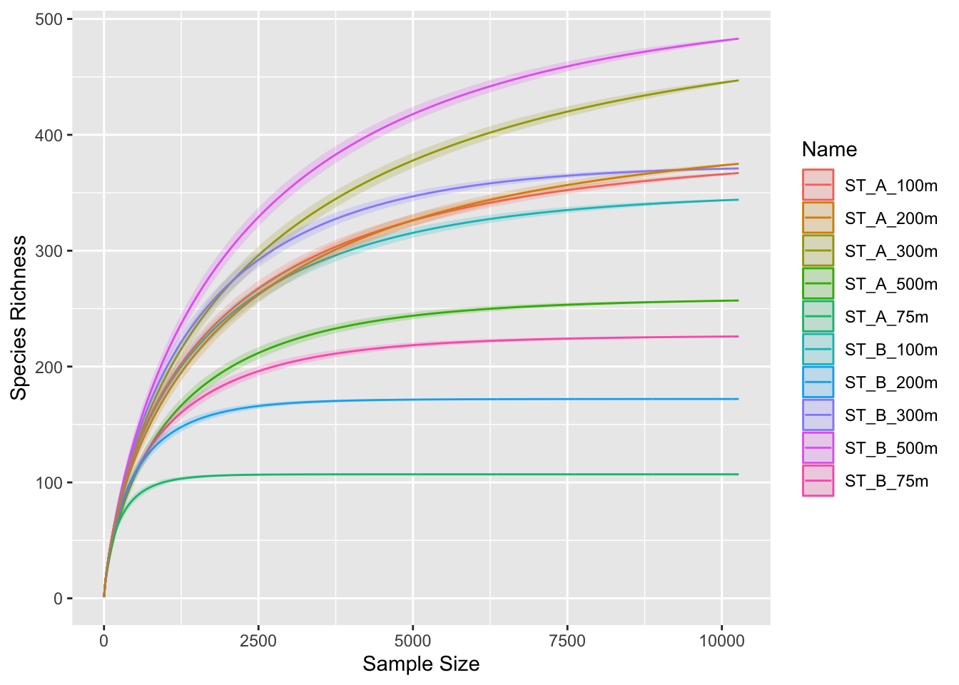
3.4 Group separation
p0 + facet_wrap(~Station, ncol = 2)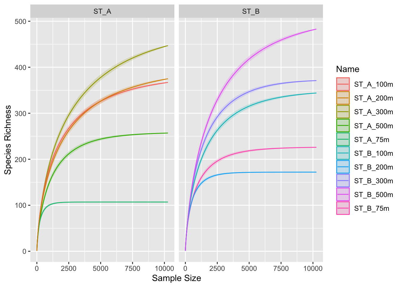
4 IV-Alpha Diversity
4.1 Indices
4.1.1 Get taxonomy-based diversity indices
#Get indices with alpha function (NB: index="all" if you want all the indices)
alpha_indices <- microbiome::alpha(
  physeq_rar,
  index = c("observed", "diversity_gini_simpson",
          "diversity_shannon", "evenness_pielou",
          "dominance_relative")
)
Observed richnessOther forms of richnessDiversityEvennessDominanceRarity#save
write.table(alpha_indices,
file = file.path(output_alpha, "indices_alpha_resultat.txt"),
sep = "\t")
#which type?
class(alpha_indices)[1] "data.frame"#see
alpha_indices observed diversity_gini_simpson diversity_shannon
barcode13_combine_Q22 447 0.9281 3.937
barcode14_combine_Q22 257 0.9108 3.564
barcode17_combine_Q22 226 0.9206 3.716
barcode18_combine_Q22 344 0.9232 3.901
barcode19_combine_Q22 172 0.9138 3.694
barcode20_combine_Q22 371 0.9079 3.811
barcode21_combine_Q22 483 0.9300 3.991
barcode22_combine_Q22 107 0.9309 3.656
barcode23_combine_Q22 367 0.9158 3.899
barcode24_combine_Q22 375 0.9331 3.935
evenness_pielou dominance_relative
barcode13_combine_Q22 0.6451 0.1964
barcode14_combine_Q22 0.6422 0.2101
barcode17_combine_Q22 0.6855 0.2357
barcode18_combine_Q22 0.6678 0.2349
barcode19_combine_Q22 0.7177 0.2545
barcode20_combine_Q22 0.6441 0.2349
barcode21_combine_Q22 0.6458 0.1833
barcode22_combine_Q22 0.7824 0.2225
barcode23_combine_Q22 0.6603 0.2519
barcode24_combine_Q22 0.6640 0.20984.1.2 Add the alpha indices result to your metadata (sample_data) phyloseq object
Important because many times you will probably want to add new variables in the phyloseq class object!!!
#Transform the alpha indices (dataframe) results into sample_data object (phyloseq) using the sample_data function
alpha_indices <- phyloseq::sample_data(alpha_indices)
#See
class(alpha_indices)
[1] "sample_data"
attr(,"package")
[1] "phyloseq"#Add alpha_indices to phyloseq sample_data object using merge_phyloseq function!
physeq_rar <- phyloseq::merge_phyloseq(physeq_rar, alpha_indices)
#See the result
sample_data(physeq_rar) SampleID Technology KIT Depth Station
barcode13_combine_Q22 barcode13_combine_Q22 Nanopore A 300m ST_A
barcode14_combine_Q22 barcode14_combine_Q22 Nanopore A 500m ST_A
barcode17_combine_Q22 barcode17_combine_Q22 Nanopore B 75m ST_B
barcode18_combine_Q22 barcode18_combine_Q22 Nanopore B 100m ST_B
barcode19_combine_Q22 barcode19_combine_Q22 Nanopore B 200m ST_B
barcode20_combine_Q22 barcode20_combine_Q22 Nanopore B 300m ST_B
barcode21_combine_Q22 barcode21_combine_Q22 Nanopore B 500m ST_B
barcode22_combine_Q22 barcode22_combine_Q22 Nanopore A 75m ST_A
barcode23_combine_Q22 barcode23_combine_Q22 Nanopore A 100m ST_A
barcode24_combine_Q22 barcode24_combine_Q22 Nanopore A 200m ST_A
Name Depths Depth_cat O2 NO3 NH4 NO2 Salinity
barcode13_combine_Q22 ST_A_300m 300 mid 128 18.5 0.94 0.11 38.32
barcode14_combine_Q22 ST_A_500m 500 deep 82 27.6 0.57 0.05 37.88
barcode17_combine_Q22 ST_B_75m 75 shallow 232 2.4 0.44 0.04 38.41
barcode18_combine_Q22 ST_B_100m 100 shallow 221 4.2 0.41 0.13 38.05
barcode19_combine_Q22 ST_B_200m 200 mid 171 10.8 0.52 0.17 37.72
barcode20_combine_Q22 ST_B_300m 300 mid 129 18.1 0.86 0.09 38.28
barcode21_combine_Q22 ST_B_500m 500 deep 82 28.5 0.43 0.03 37.95
barcode22_combine_Q22 ST_A_75m 75 shallow 228 2.0 0.40 0.06 38.10
barcode23_combine_Q22 ST_A_100m 100 shallow 208 4.8 0.69 0.11 37.83
barcode24_combine_Q22 ST_A_200m 200 mid 166 9.9 0.98 0.19 38.36
pH Turbidity Pollutant observed diversity_gini_simpson
barcode13_combine_Q22 8.06 1.8 9.44 447 0.9281
barcode14_combine_Q22 7.98 2.1 9.33 257 0.9108
barcode17_combine_Q22 8.12 1.5 9.30 226 0.9206
barcode18_combine_Q22 8.03 2.3 9.30 344 0.9232
barcode19_combine_Q22 7.95 1.9 9.00 172 0.9138
barcode20_combine_Q22 8.10 2.0 8.84 371 0.9079
barcode21_combine_Q22 8.01 1.7 8.57 483 0.9300
barcode22_combine_Q22 7.92 2.2 9.74 107 0.9309
barcode23_combine_Q22 8.08 1.6 9.83 367 0.9158
barcode24_combine_Q22 8.00 1.8 9.66 375 0.9331
diversity_shannon evenness_pielou dominance_relative
barcode13_combine_Q22 3.937 0.6451 0.1964
barcode14_combine_Q22 3.564 0.6422 0.2101
barcode17_combine_Q22 3.716 0.6855 0.2357
barcode18_combine_Q22 3.901 0.6678 0.2349
barcode19_combine_Q22 3.694 0.7177 0.2545
barcode20_combine_Q22 3.811 0.6441 0.2349
barcode21_combine_Q22 3.991 0.6458 0.1833
barcode22_combine_Q22 3.656 0.7824 0.2225
barcode23_combine_Q22 3.899 0.6603 0.2519
barcode24_combine_Q22 3.935 0.6640 0.20984.2 Alpha diversity representations
This section will show you how to plot by different ways the alpha diversity and its customization. Understand how it works!
4.2.1 Alpha representations using phyloseq::plot_richness()
You are limited to the indices calculated by the phyloseq::estimate_richness function (i.e.”Observed”, “Chao1”, “ACE”, “Shannon”, “Simpson”, “InvSimpson”, “Fisher”).
4.2.1.1 Selected indices + Name
x allow you to choose the column from sample_data(physeq_rar) for applying the label
phyloseq::plot_richness(physeq_rar, x = "SampleID",
                        measures = c("Observed", "Shannon", "Simpson"))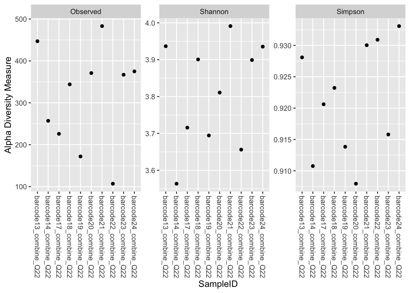
4.2.2 Color by group: color = Station & change sample name
For color option pass the column of sample_data(physeq_rar) that you want. Here different colors is applied depending on Station (which is A and B, so 2 different colors)
phyloseq::plot_richness(physeq_rar,
                        x = "Name",
                        color="Station",
                        measures=c("Observed", "Shannon", "Simpson"))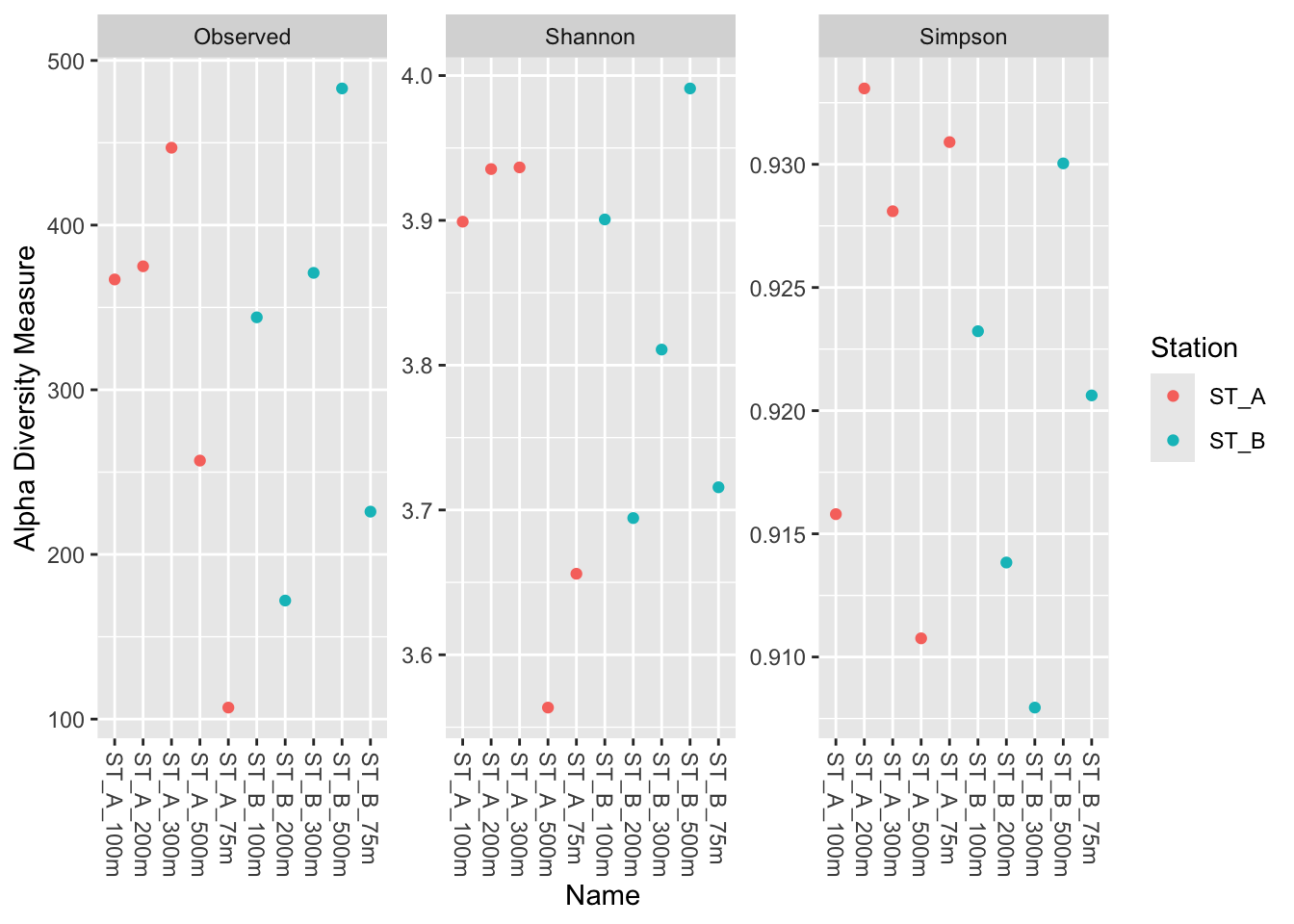
4.2.3 Make box_plot by adding geom_boxplot function
phyloseq::plot_richness(physeq_rar,
                        x="Station",
                        color="Station",
                        measures=c("Observed", "Shannon", "Simpson")) +
  ggplot2::geom_boxplot()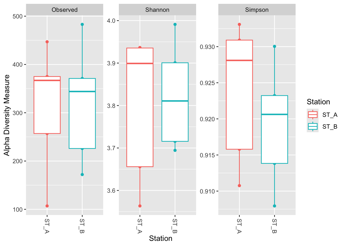
4.2.4 Make box_plot : geom_boxplot + fill color of boxplot (fill) + transparency (with alpha)
phyloseq::plot_richness(physeq_rar,
                        x = "Station",
                        measures = c("Observed", "Shannon", "Simpson")) +
geom_boxplot(aes(fill = Station), alpha = 0.4, color = "gray40", linewidth = 0.3)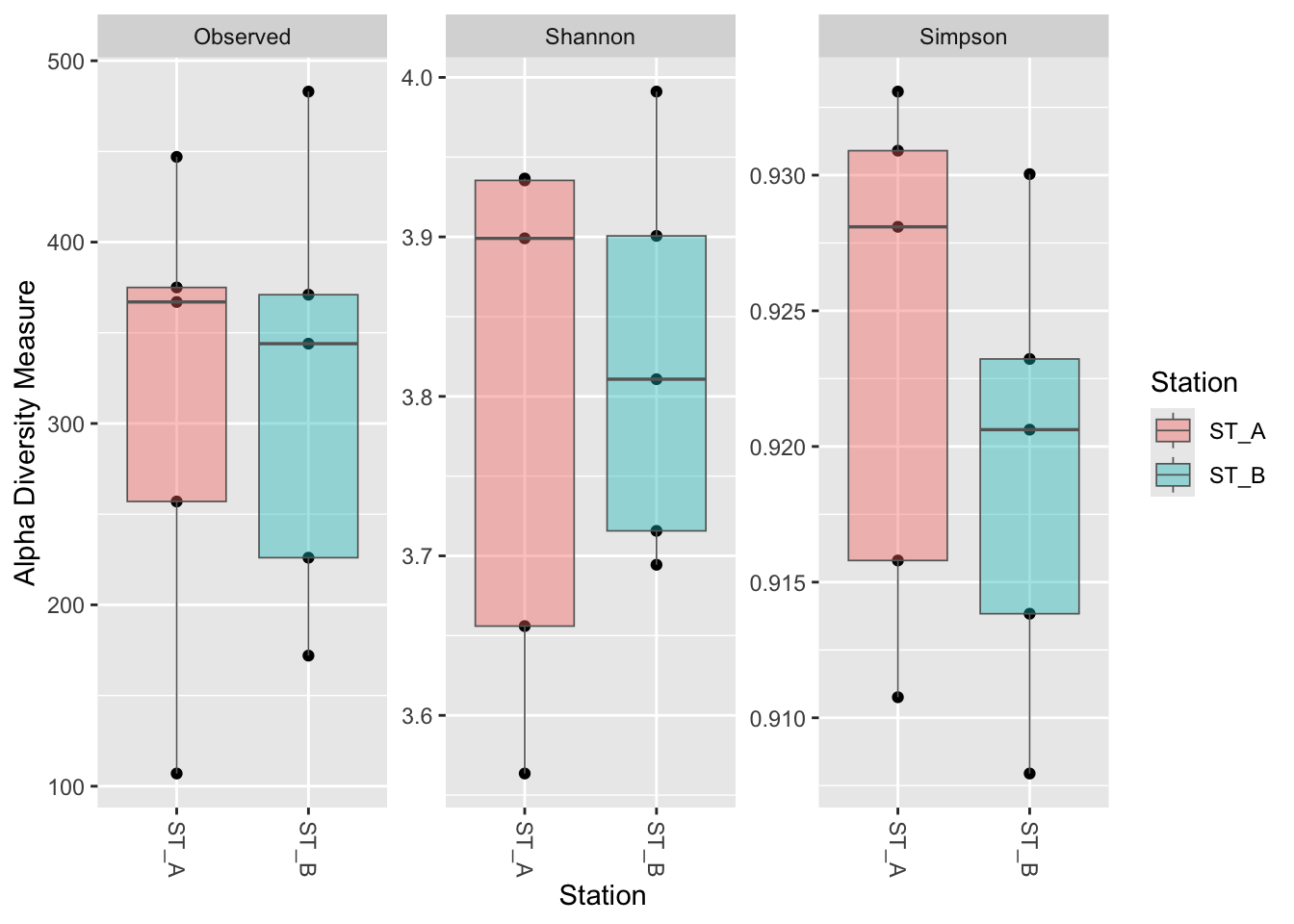
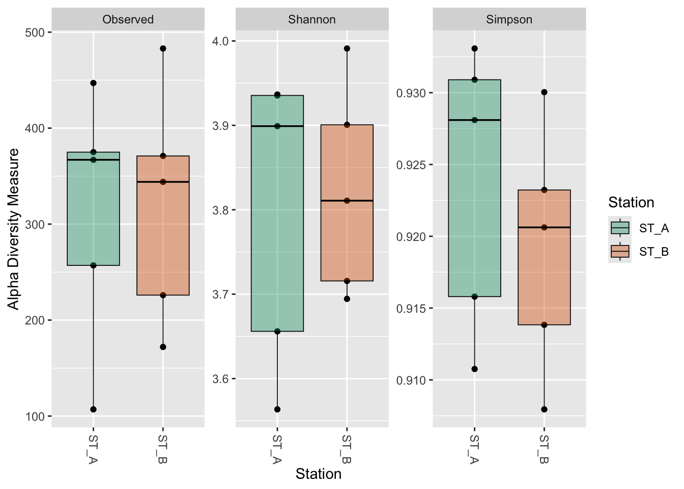
4.2.5 Make box_plot : geom_boxplot + scale_fill_manual
phyloseq::plot_richness(
    physeq_rar,
    x = "Station",
    measures = c("Observed", "Shannon", "Simpson")
) +
    geom_boxplot(aes(fill = Station), alpha = 0.4, color = "black", linewidth = 0.3) +
    scale_fill_manual(
        values = c(
            "ST_A" = "#1b9e77",
            "ST_B" = "#d95f02"
        )
    )
4.2.6 Alpha representations using
Microbiome::boxplot_alpha (not shown)
Again, you are limited to the indices calculated by the Microbiome::alpha function
#Before : Change your phyloseq class oject sample_data as a dataframe
metadata <- data.frame(sample_data(physeq_rar))
head(metadata)
SampleID Technology KIT Depth Station
barcode13_combine_Q22 barcode13_combine_Q22 Nanopore A 300m ST_A
barcode14_combine_Q22 barcode14_combine_Q22 Nanopore A 500m ST_A
barcode17_combine_Q22 barcode17_combine_Q22 Nanopore B 75m ST_B
barcode18_combine_Q22 barcode18_combine_Q22 Nanopore B 100m ST_B
barcode19_combine_Q22 barcode19_combine_Q22 Nanopore B 200m ST_B
barcode20_combine_Q22 barcode20_combine_Q22 Nanopore B 300m ST_B
Name Depths Depth_cat O2 NO3 NH4 NO2 Salinity
barcode13_combine_Q22 ST_A_300m 300 mid 128 18.5 0.94 0.11 38.32
barcode14_combine_Q22 ST_A_500m 500 deep 82 27.6 0.57 0.05 37.88
barcode17_combine_Q22 ST_B_75m 75 shallow 232 2.4 0.44 0.04 38.41
barcode18_combine_Q22 ST_B_100m 100 shallow 221 4.2 0.41 0.13 38.05
barcode19_combine_Q22 ST_B_200m 200 mid 171 10.8 0.52 0.17 37.72
barcode20_combine_Q22 ST_B_300m 300 mid 129 18.1 0.86 0.09 38.28
pH Turbidity Pollutant observed diversity_gini_simpson
barcode13_combine_Q22 8.06 1.8 9.44 447 0.9281
barcode14_combine_Q22 7.98 2.1 9.33 257 0.9108
barcode17_combine_Q22 8.12 1.5 9.30 226 0.9206
barcode18_combine_Q22 8.03 2.3 9.30 344 0.9232
barcode19_combine_Q22 7.95 1.9 9.00 172 0.9138
barcode20_combine_Q22 8.10 2.0 8.84 371 0.9079
diversity_shannon evenness_pielou dominance_relative
barcode13_combine_Q22 3.937 0.6451 0.1964
barcode14_combine_Q22 3.564 0.6422 0.2101
barcode17_combine_Q22 3.716 0.6855 0.2357
barcode18_combine_Q22 3.901 0.6678 0.2349
barcode19_combine_Q22 3.694 0.7177 0.2545
barcode20_combine_Q22 3.811 0.6441 0.23494.2.7 Alpha representations using ggplot2
Interest: Freedom!! you can use ANY indices that you have calculated from different packages & included in sample_data 4.2.6.1 Boxplot, color control, points and Mean SD: stat_summary()
ggplot(metadata, aes(x = Station, y = observed)) +
  geom_boxplot(alpha = 0.6,
               fill = c("#00AFBB", "#E7B800"),
               color=c("#00AFBB", "#E7B800")) +
  geom_jitter(aes(colour = Depth_cat), position = position_jitter(0.07), cex = 2.2) +
  stat_summary(fun = mean, geom = "point", shape = 17, size = 3, color = "white") +
  stat_summary(fun.data = "mean_se", geom = "errorbar", width = .1, color = "white")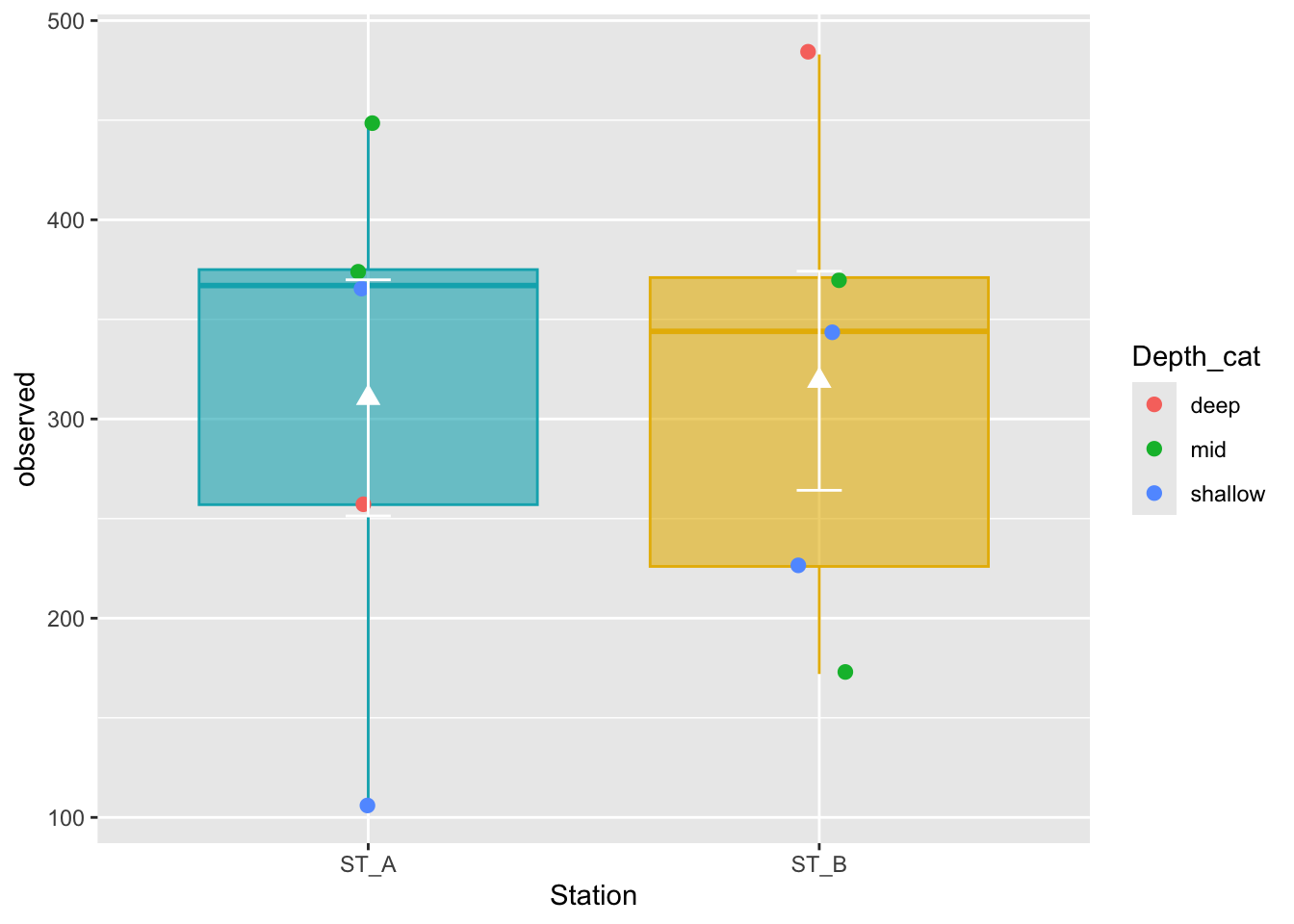
4.2.8 Combine graphs on same figure: patchwork
#Put your  graphs in different variables P1,P2,P3
p1 <- ggplot(metadata, aes(x = Station, y = observed)) +
  geom_boxplot(alpha = 0.6,
               fill = c("#00AFBB","#E7B800"),
               color=c("#00AFBB","#E7B800")) +
  geom_jitter(aes(colour = Depth_cat), position = position_jitter(0.07), cex = 2.2) +
  theme(axis.title.x = element_blank())

p2 <- ggplot(metadata, aes(x = Station, y = evenness_pielou)) +
  geom_boxplot(alpha = 0.6,
               fill = c("#00AFBB", "#E7B800"),
               color = c("#00AFBB", "#E7B800")) +
  geom_jitter(aes(colour = Depth_cat), position = position_jitter(0.07), cex = 2.2) +
  theme(axis.title.x = element_blank())

p3 <- ggplot(metadata, aes(x = Station, y = diversity_gini_simpson)) +
  geom_boxplot(alpha = 0.6,
               fill = c("#00AFBB", "#E7B800"),
               color = c("#00AFBB", "#E7B800")) +
  geom_jitter(aes(colour = Depth_cat), position = position_jitter(0.07), cex = 2.2) +
  theme(axis.title.x = element_blank())
#Put the graph of p1, p2 and p3 on same Figure
p1 + p2 + p3 +
patchwork::plot_annotation(tag_levels = "A") +
patchwork::plot_layout(guides = "collect")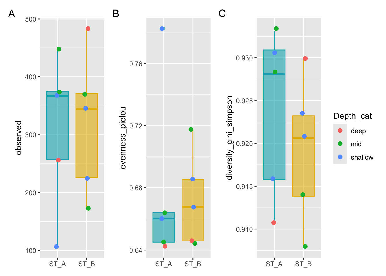
5 Statistical hypothesis for alpha diversity
The goal here is to illustrate the statistical methods; however, the sampling design is too limited to support strong conclusions
5.1 Normality test: Check the normal or not normal distribution of your data to choose the right test!
5.1.2 Shapiro test: H0 Null Hypothesis: follows Normal distribution!
Means if p<0.05 -> reject the H0 (so does not follow a normal distribution)
5.1.3 Q-Qplots: Compare your distribution with a theoretical normal distribution
If your data follow a normal distribution, you’re expecting a linear relationship theoritical vs.experimental
Our custom function indices_normality() (defined in R/alpha_diversity.R) plots the results of Shapiro test as well as Q-Qplots.
5.1.4 Select indices to test & run normality check
metadata |>
  dplyr::select(observed,
                diversity_gini_simpson,
                diversity_shannon,
                evenness_pielou) |>
  indices_normality(nrow = 3, ncol = 2)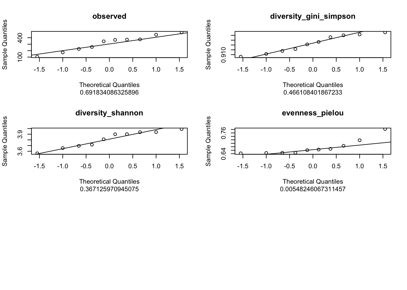
What are your conclusion about the normality of each index?
5.2 ANOVA: parametric (follows normal distribution) AND at least 3 groups
5.2.1 Anova for Observed richness and 3 groups (Depth_cat)
# How many groups used? See the column "groupe" of metadata:
factor(metadata$Depth_cat)
[1] mid deep shallow shallow mid mid deep shallow shallow
[10] mid
Levels: deep mid shallow5.2.2 Variance
# Check homogeneity of variance between groups
# (avoid bias in ANOVA result & keep the power of the test)
# H0= equality of variances in the different populations
stats::bartlett.test(observed ~ Depth_cat, metadata)
    Bartlett test of homogeneity of variances

data:  observed by Depth_cat
Bartlett's K-squared = 0.14, df = 2, p-value = 0.9
Conclusion?
NB : Alternative to Bartlett : Levene test (package car), less sensitive to normality deviation
5.2.3 Anova
Global Test: Anova tell you if that some of the group means are different, but you don’t know which pairs of groups are different!
aov_observed <- stats::aov(observed ~ Depth_cat, metadata)
summary(aov_observed)
Df Sum Sq Mean Sq F value Pr(>F)
Depth_cat 2 20470 10235 0.65 0.55
Residuals 7 110457 15780 5.2.4 Which pairs of groups are different? -> Post-hoc test: Tukey multiple pairwise-comparisons
signif_pairgroups <- stats::TukeyHSD(aov_observed, method = "bh")
signif_pairgroups
Tukey multiple comparisons of means
95% family-wise confidence level
Fit: stats::aov(formula = observed ~ Depth_cat, data = metadata)
$Depth_cat
diff lwr upr p adj
mid-deep -28.75 -349.1 291.6 0.9624
shallow-deep -109.00 -429.4 211.4 0.5988
shallow-mid -80.25 -341.8 181.3 0.6554What is our mistake ?
5.3 Kruskal-Wallis: non-parametric & at least three groups
5.3.1 Global test
stats::kruskal.test(evenness_pielou ~ Depth_cat, data = metadata)
    Kruskal-Wallis rank sum test

data:  evenness_pielou by Depth_cat
Kruskal-Wallis chi-squared = 3.8, df = 2, p-value = 0.1
5.3.2 Post hoc test: Dunn test (pairwise group test)
signifgroup <- FSA::dunnTest(evenness_pielou ~ Depth_cat,
                           data = metadata,
                           method = "bh")
#See
signifgroupDunn (1964) Kruskal-Wallis multiple comparison p-values adjusted with the Benjamini-Hochberg method. Comparison Z P.unadj P.adj
1 deep - mid -0.9535 0.34036 0.3404
2 deep - shallow -1.9069 0.05653 0.1696
3 mid - shallow -1.1677 0.24291 0.36445.4 T-test: parametric, 2 groups (i.e Station A vs B)
5.4.1 Variance homogeneity
stats::bartlett.test(observed ~ Station, metadata)
    Bartlett test of homogeneity of variances

data:  observed by Station
Bartlett's K-squared = 0.02, df = 1, p-value = 0.9
5.4.2 t-test
observed_ttest <- stats::t.test(observed ~ Station, data = metadata)
#see
observed_ttest
Welch Two Sample t-test
data: observed by Station
t = -0.11, df = 8, p-value = 0.9
alternative hypothesis: true difference in means between group ST_A and group ST_B is not equal to 0
95 percent confidence interval:
-195.2 178.0
sample estimates:
mean in group ST_A mean in group ST_B
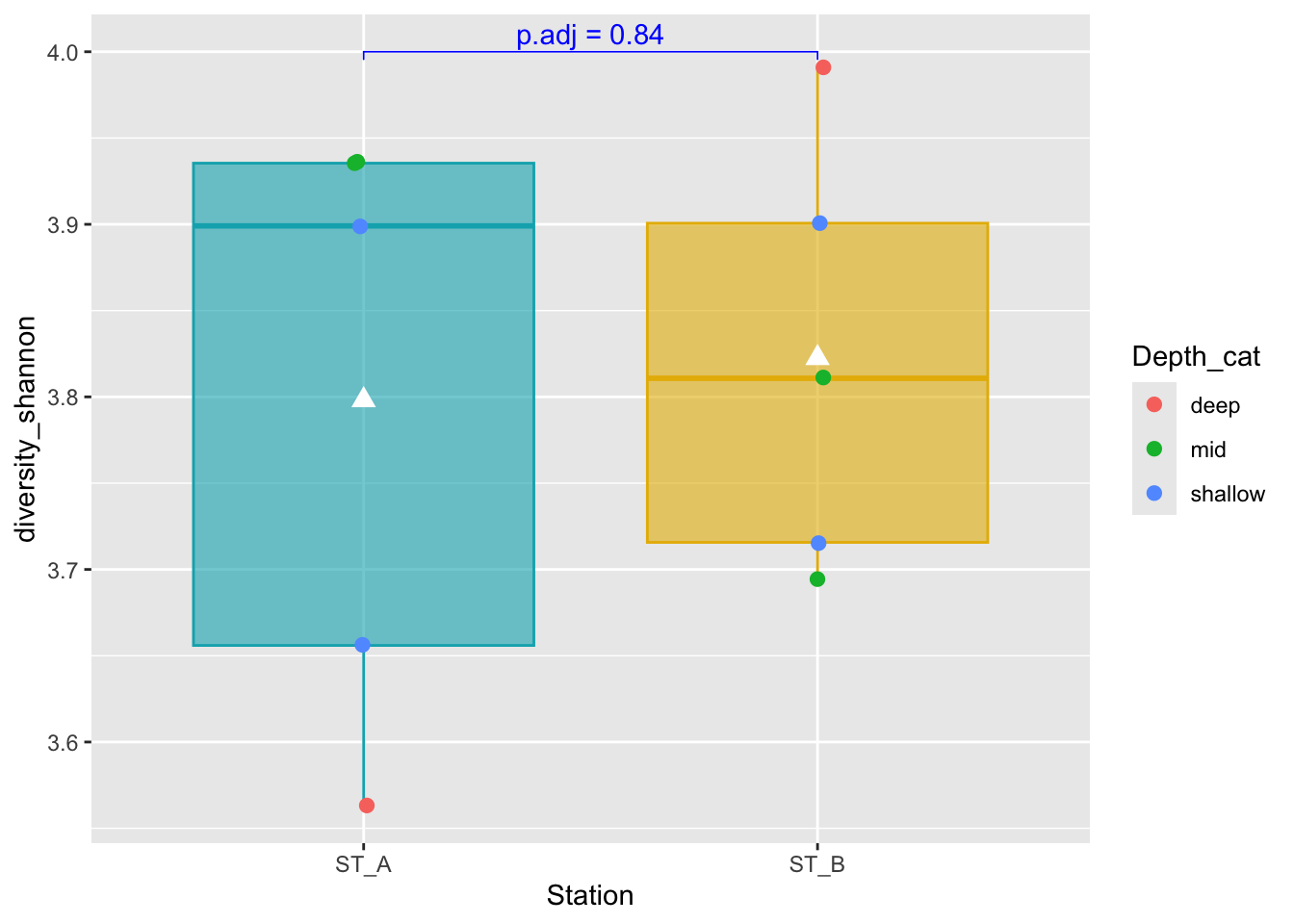
310.6 319.2 5.5 Wilcoxon rank sum: non-parametric & 2 Groups
pairwise_test <- ggpubr::compare_means( diversity_shannon ~ Station,
                                       metadata,
                                       method = "wilcox.test")
Registered S3 methods overwritten by 'car':
method from
hist.boot FSA
confint.boot FSA #See
pairwise_test# A tibble: 1 × 8
.y. group1 group2 p p.adj p.format p.signif method
<chr> <chr> <chr> <dbl> <dbl> <chr> <chr> <chr>
1 diversity_shannon ST_A ST_B 0.841 0.84 0.84 ns WilcoxonWhat is the mistake here ?
5.5.1 Boxplot representation with p-value information
#Boxplot as previously seen
graph_shan <- ggplot(metadata, aes(x = Station, y = diversity_shannon)) +
  geom_boxplot(alpha=0.6,
               fill = c("#00AFBB", "#E7B800"),
               color = c("#00AFBB", "#E7B800")) +
  geom_jitter(aes(colour = Depth_cat),
              position = position_jitter(0.02) ,
              cex=2.2)+
  stat_summary(fun = mean, geom = "point",
               shape = 17, size = 3,
               color = "white")

#Add p-value on graph
graph_shan + ggpubr::stat_pvalue_manual(
  pairwise_test,
  y.position = 4,
  label = "p.adj = {p.adj}",
  color = "blue",
  linetype = 1,
  tip.length = 0.01
)
6 Taxonomy: barplot graph
6.1 Abundance Transformation
6.1.1 Counts in percentage using phyloseq::transform_sample_counts()
pourcentS <- phyloseq::transform_sample_counts(physeq_rar, function(x) x/sum(x) * 100)See Plot
phyloseq::plot_bar(pourcentS)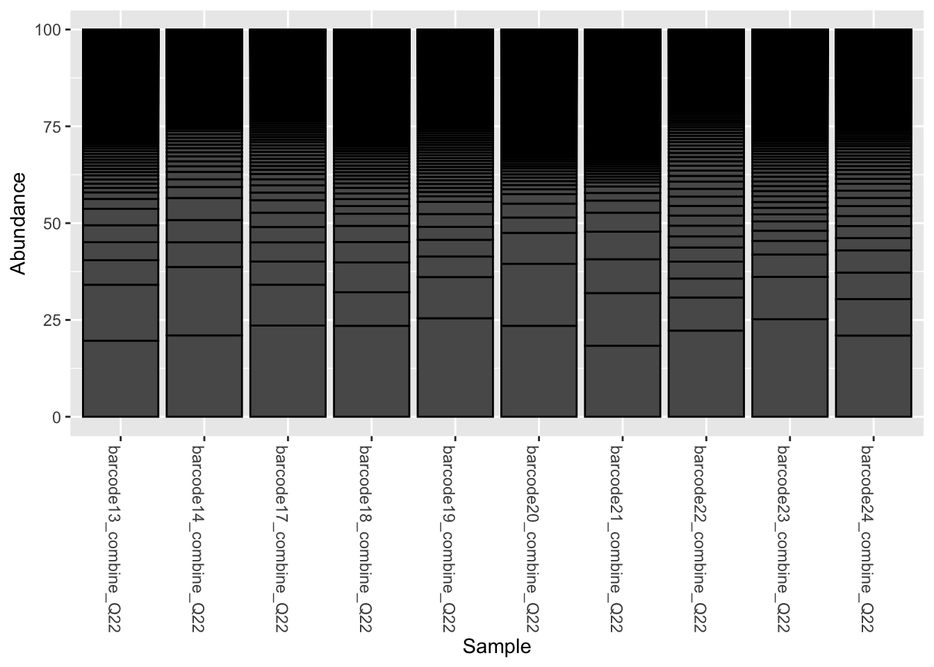
What are the separation lines?
6.1.2 Summarise at a given taxonomic level with phyloseq::tax_glom()
Remember ranks can be obtained with phyloseq::rank_names()
phyloseq::rank_names(pourcentS)[1] "kingdom" "phylum" "class" "order" "family" "genus" "species"Phylum_glom <- phyloseq::tax_glom(pourcentS,
taxrank = "phylum",
NArm = FALSE)
#Plot at Phylum taxonomic rank, with color
phyloseq::plot_bar(Phylum_glom, fill = "phylum") 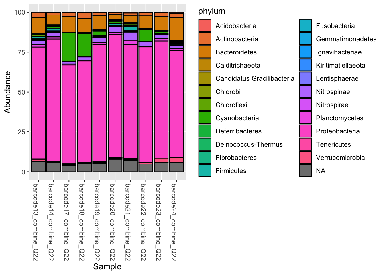
NArm what for?
6.1.3 Filter phylum (mean of the line): phyloseq::filter_taxa()
Let’s filter out the phylums with a mean relative abundance inferior to 1%
Phylum_1 <- phyloseq::filter_taxa(Phylum_glom,
                                  flist = function(x) mean(x) >= 1,
                                  prune = TRUE)

#Plot at Phylum taxonomic rank, with color
phyloseq::plot_bar(Phylum_1, fill = "phylum") 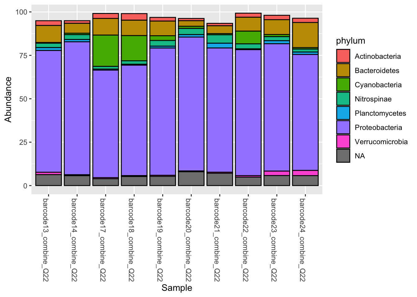
6.1.4 How to save a table into a file: exemple of phylum taxonomic table
write.table(df_export(otu_table(Phylum_glom)),
            row.names = FALSE,
            file = file.path(output_alpha, "Phylum_pourcent.tsv"),
            sep = "\t")
6.1.5 Remove black lines
phyloseq::plot_bar(Phylum_glom, "Name", fill = "phylum") +
  geom_bar(aes(colour = phylum), stat = "identity")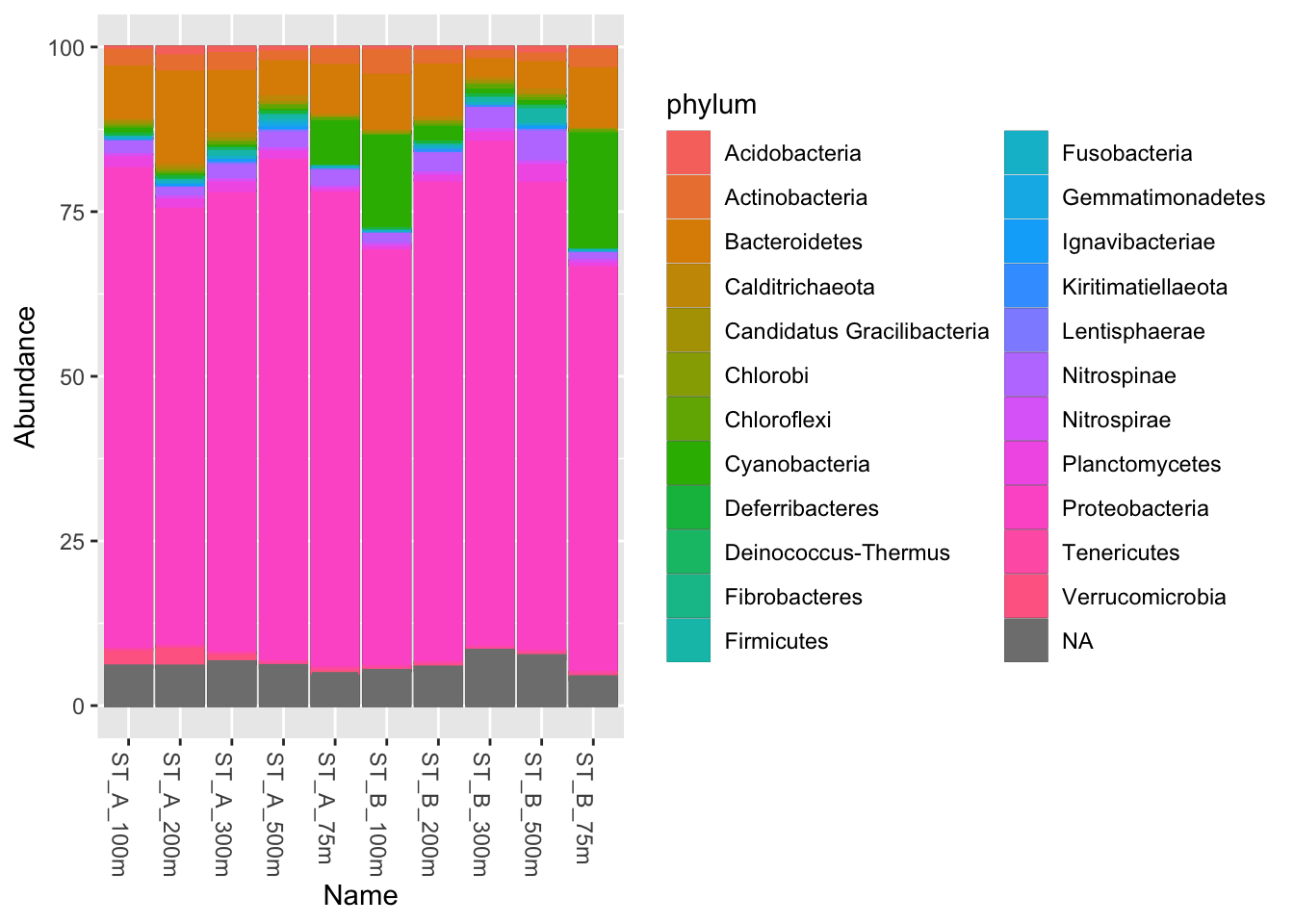
6.2 Microbiome package
6.2.1 microbiome::aggregate_taxa()
# Order Rank
Order_microb <- microbiome::aggregate_taxa(pourcentS, "order")

#Filter at 1%
Order1 <- phyloseq::filter_taxa(Order_microb, function(x) mean(x) >= 1, prune = TRUE)
6.2.2 microbiome::plot_composition()
p_order <- microbiome::plot_composition(Order1,
                                        otu.sort = "abundance",
                                        sample.sort = "Name",
                                        x.label = "Name",
                                        plot.type = "barplot",
                                        verbose = FALSE) +
  ggplot2::labs(x = "", y = "Relative abundance (%)")
#see
p_order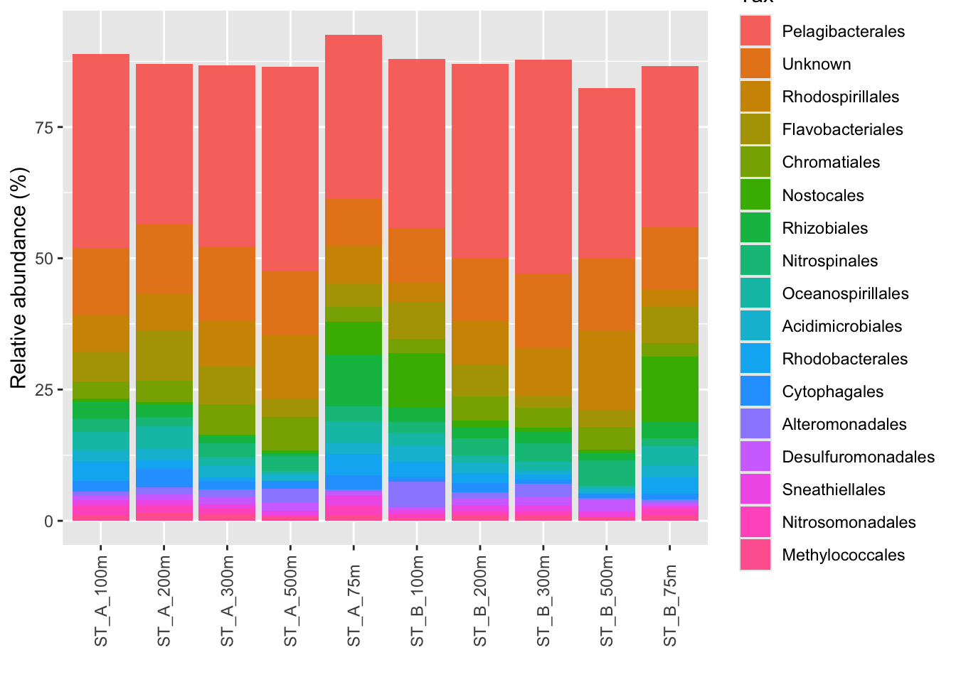
6.2.3 Change the order of X- axis label
#definir l'ordre
ordre_voulu <- c(
  "ST_A_75m", "ST_A_100m", "ST_A_200m", "ST_A_300m", "ST_A_500m",
  "ST_B_75m", "ST_B_100m", "ST_B_200m", "ST_B_300m", "ST_B_500m"
)
# levels -> prends dans l'ordre que je donne
sample_data(Order1)$Name <- factor(
  sample_data(Order1)$Name,
  levels = ordre_voulu
)
p_order1 <- microbiome::plot_composition(Order1,
otu.sort = "abundance",
sample.sort = "Name",
x.label = "Name",
plot.type = "barplot",
verbose = FALSE) +
ggplot2::labs(x = "", y = "Relative abundance (%)")
#see
p_order1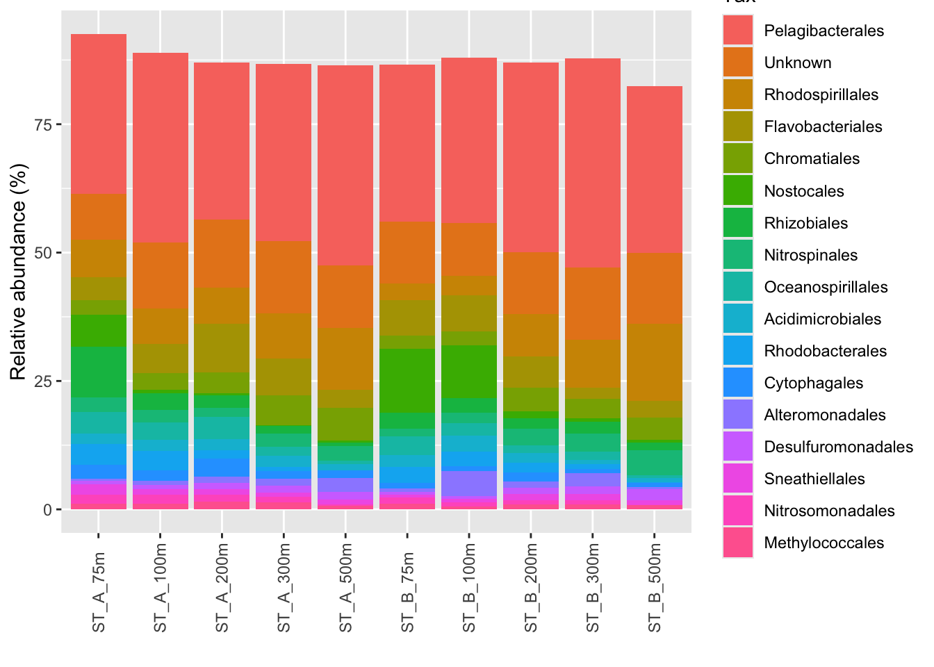
#Average by group :average_by option
p_order_groupe <- microbiome::plot_composition(Order1,
                                               otu.sort = "abundance",
                                               sample.sort = "Name",
                                               x.label = "Name",
                                               plot.type = "barplot",
                                               verbose = FALSE,
                                               average_by = "Station") +
  ggplot2::labs(x = "", y = "Relative abundance (%)")

#see
p_order_groupe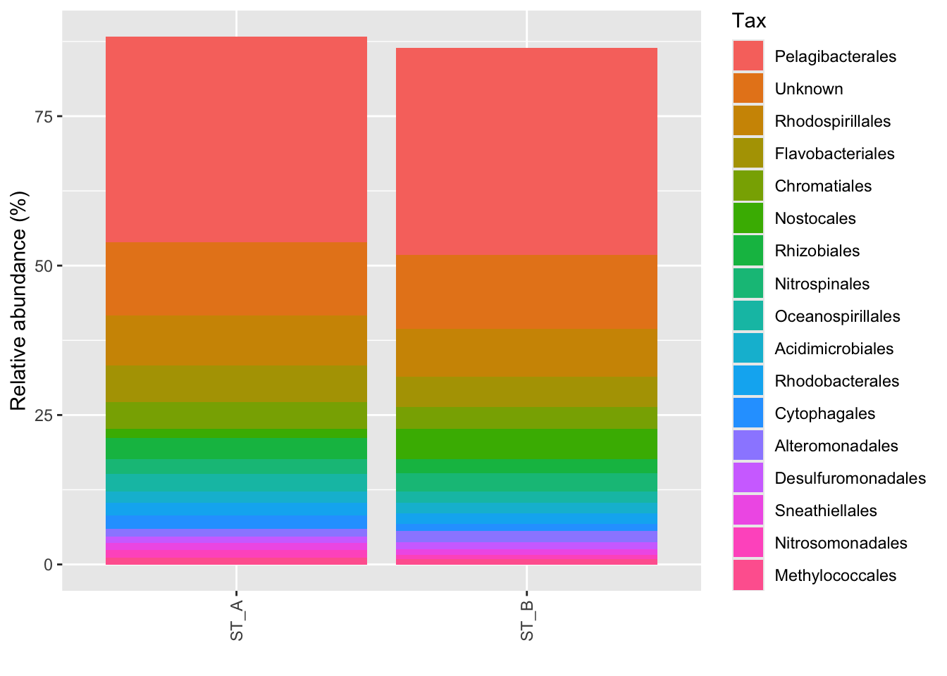
6.2.4 Interactive barplot with plotly::ggplotly()
plotly::ggplotly(p_order)6.2.5 How to manage colors in barplots
With the number of Phyla, Order etc a barplot can become very confusing… Need to have distinct color for each taxonomic groups.
Use the library RColorBrewer et scale_fill_manual() See here to understand the possibilities
You can visualise RColorBrewer’s palettes with the following command:
RColorBrewer::display.brewer.all()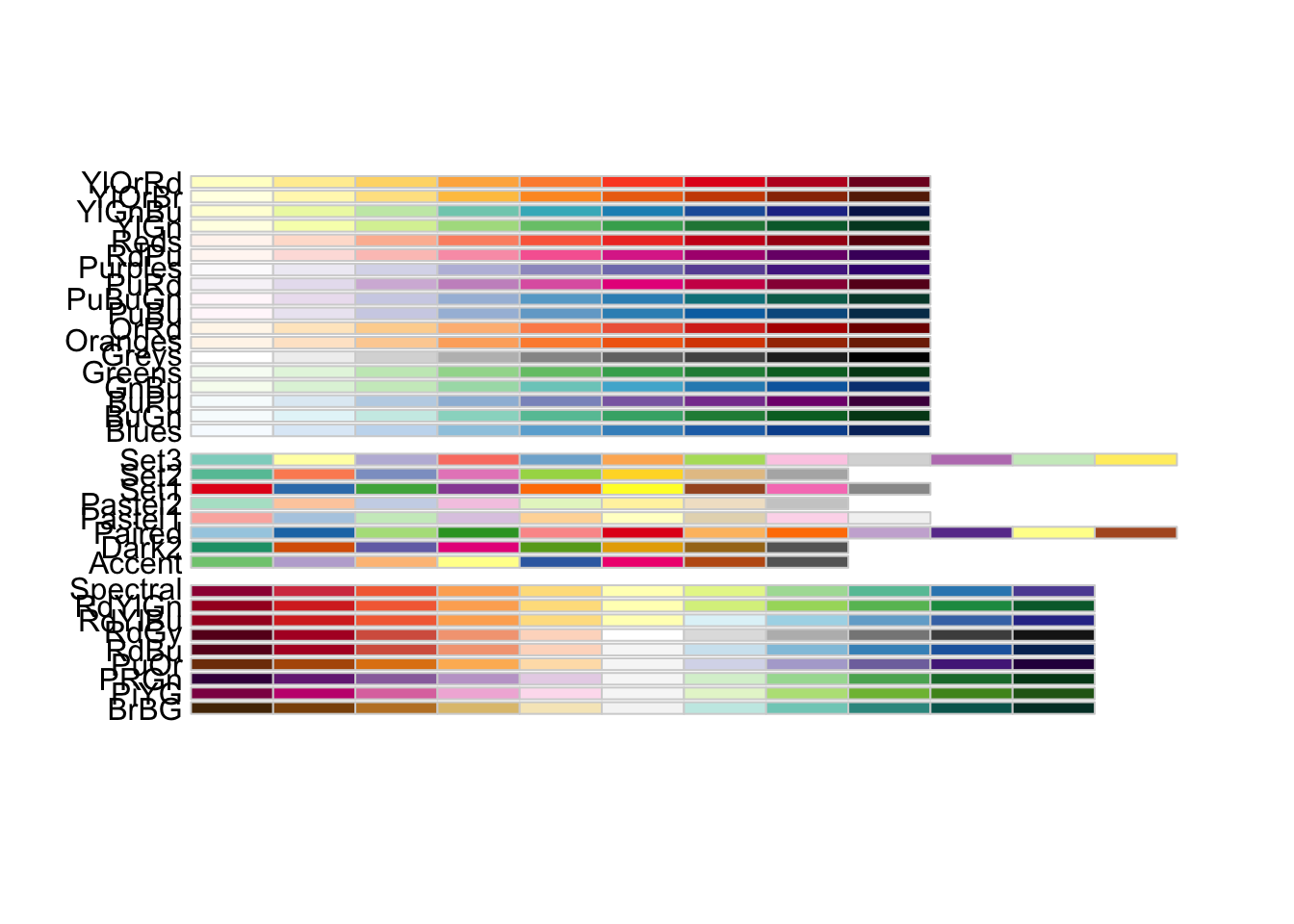
6.2.6 Build your own palette
Let’s assemble from two RColorBrewer’s palettes a single 13 colors palette
#See Set2 colors
(col1 <- RColorBrewer::brewer.pal(name = "Set2", n = 8))
[1] "#66C2A5" "#FC8D62" "#8DA0CB" "#E78AC3" "#A6D854" "#FFD92F" "#E5C494"
[8] "#B3B3B3"#See Paired colors
(col2 <- RColorBrewer::brewer.pal(name = "Paired", n = 10)) [1] "#A6CEE3" "#1F78B4" "#B2DF8A" "#33A02C" "#FB9A99" "#E31A1C" "#FDBF6F"
[8] "#FF7F00" "#CAB2D6" "#6A3D9A"#Build your set of colors using brewer.pal or your own colors
mycolors <- c(col1, col2)6.2.7 Use your palette in the p_order barplot
#Use scale_fill_manual
p_order +
  ggplot2::scale_fill_manual("Order", values = mycolors) +
  theme(legend.position = "right",
        legend.text = element_text(size=8))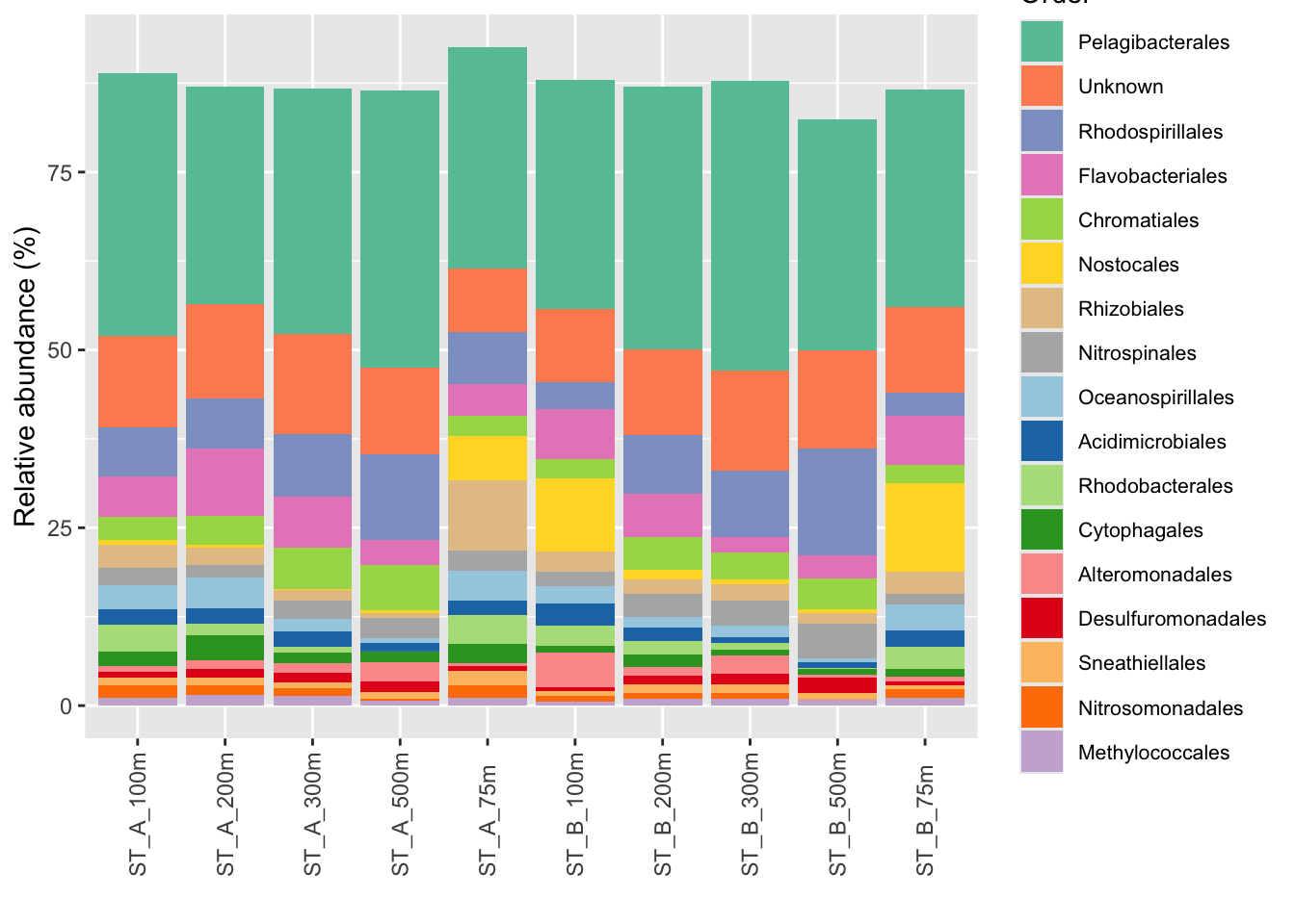
6.2.8 To go even further in choosing colors
See ANF : https://anf-metabiodiv.github.io/course-material/practicals/alpha_diversity.html
6.3 Other data Manipulation : select specific taxa, merge samples
6.3.1 Select Actinobacteria AND Bacteroidetes: phyloseq::subset_taxa()
myselection1 <- phyloseq::subset_taxa(Phylum_glom, phylum == "Actinobacteria" | phylum == "Bacteroidetes")

phyloseq::plot_bar(myselection1, x = "Name", fill = "phylum")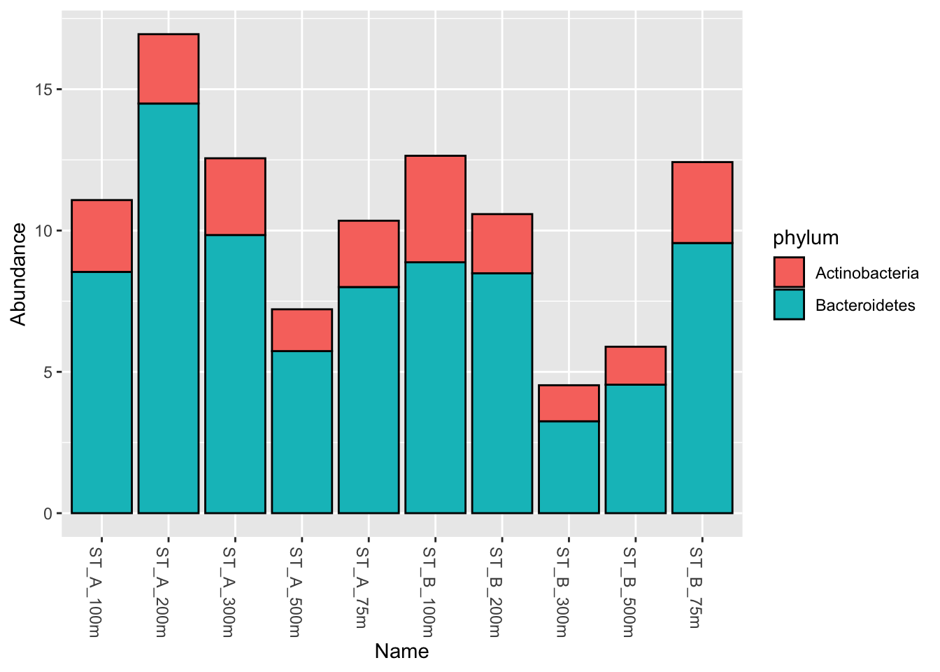
phyloseq::plot_bar(myselection1, x = "Name",
fill="phylum", facet_grid = ~phylum) 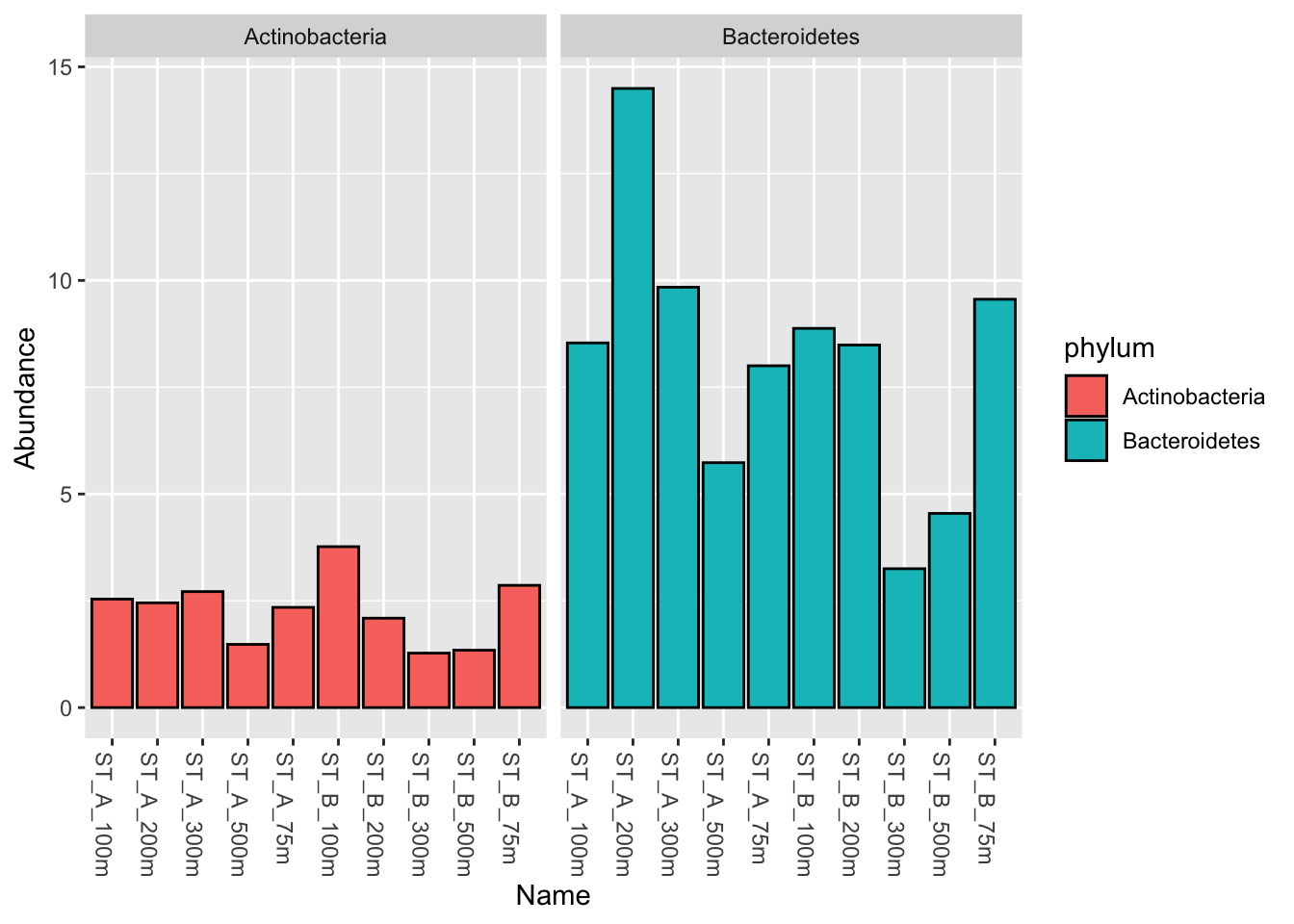
6.3.2 Keep all with the exception of a class, a genus etc (e.g.contamination)
myselection2 <- phyloseq::subset_taxa(physeq_rar, class != "Cytophagia" | is.na(class))
myselection2
phyloseq-class experiment-level object
otu_table() OTU Table: [ 788 taxa and 10 samples ]
sample_data() Sample Data: [ 10 samples by 21 sample variables ]
tax_table() Taxonomy Table: [ 788 taxa by 7 taxonomic ranks ]
refseq() DNAStringSet: [ 788 reference sequences ]6.3.3 Understand:
! = means IS NOT
| = AND
Is.na = do not remove the NA (Not Assigned at the Class rank), by default it will be removed. be careful!
6.3.4 Merge samples (groups, duplicates etc)
Use a column from metadata to group/merge samples (Station A & B)
(STA_merge <- phyloseq::merge_samples(physeq_rar, "Station"))phyloseq-class experiment-level object
otu_table() OTU Table: [ 802 taxa and 2 samples ]
sample_data() Sample Data: [ 2 samples by 21 sample variables ]
tax_table() Taxonomy Table: [ 802 taxa by 7 taxonomic ranks ]6.3.5 Sample selection: phyloseq::subset_samples()
(sub_StationA <- phyloseq::subset_samples(pourcentS, Station == "ST_A"))phyloseq-class experiment-level object
otu_table() OTU Table: [ 802 taxa and 5 samples ]
sample_data() Sample Data: [ 5 samples by 21 sample variables ]
tax_table() Taxonomy Table: [ 802 taxa by 7 taxonomic ranks ]
refseq() DNAStringSet: [ 802 reference sequences ]6.3.6 Alternative way: phyloseq::prune_samples
Define what you want to keep
keep <- c("barcode17_combine_Q22", "barcode18_combine_Q22")Then extract these samples from pourcentS phyloseq object
keep2samples <- phyloseq::prune_samples(keep, pourcentS)
sample_names(keep2samples)
[1] "barcode17_combine_Q22" "barcode18_combine_Q22"6.4 Retrieve sequences from a phyloseq object
6.4.1 One sequence :
Biostrings::writeXStringSet(physeq_rar@refseq["1450761"],
                            filepath = file.path(output_alpha,"1450761.fasta"),
                            format = "fasta")
6.4.2 By name :
listsp <- c("1495650", "1496", "1505037", "1476")Biostrings::writeXStringSet(physeq_rar@refseq[listsp],
filepath = file.path(output_alpha,"several_species.fasta"),
format = "fasta")6.4.3 From a selection :
Let’s export a fasta files of all species with a maximum relative abundance superior to 10% in Station A samples:
phyloseq::subset_samples(pourcentS, Station == "ST_A") |>
  phyloseq::filter_taxa(flist = function(x) max(x) >= 10, prune = TRUE) |>
  phyloseq::refseq() |>
  Biostrings::writeXStringSet(
    filepath = file.path(output_alpha, "fancy_selection_sp.fasta"),
    format = "fasta"
  )
6.4.4 Retrieve all sequences
Biostrings::writeXStringSet(physeq_rar@refseq,
                            filepath = file.path(output_alpha,"all_sp.fasta"),
                            format = "fasta")
7 Core microbiota analysis
7.1 Which core? Compare Station A & Station B core microbiota
First start with Station A
#Create 2 phyloseq objects for North and South sample groups
sub_StA <- phyloseq::subset_samples(pourcentS, Station == "ST_A")
sub_StA
phyloseq-class experiment-level object
otu_table() OTU Table: [ 802 taxa and 5 samples ]
sample_data() Sample Data: [ 5 samples by 21 sample variables ]
tax_table() Taxonomy Table: [ 802 taxa by 7 taxonomic ranks ]
refseq() DNAStringSet: [ 802 reference sequences ]# 2. Enlever les taxa avec uniquement des zéros
sub_StA <- phyloseq::prune_taxa(taxa_sums(sub_StA) > 0, sub_StA)
sub_StAphyloseq-class experiment-level object
otu_table() OTU Table: [ 595 taxa and 5 samples ]
sample_data() Sample Data: [ 5 samples by 21 sample variables ]
tax_table() Taxonomy Table: [ 595 taxa by 7 taxonomic ranks ]
refseq() DNAStringSet: [ 595 reference sequences ]#Check group Station A ok
sub_StA@sam_data SampleID Technology KIT Depth Station
barcode13_combine_Q22 barcode13_combine_Q22 Nanopore A 300m ST_A
barcode14_combine_Q22 barcode14_combine_Q22 Nanopore A 500m ST_A
barcode22_combine_Q22 barcode22_combine_Q22 Nanopore A 75m ST_A
barcode23_combine_Q22 barcode23_combine_Q22 Nanopore A 100m ST_A
barcode24_combine_Q22 barcode24_combine_Q22 Nanopore A 200m ST_A
Name Depths Depth_cat O2 NO3 NH4 NO2 Salinity
barcode13_combine_Q22 ST_A_300m 300 mid 128 18.5 0.94 0.11 38.32
barcode14_combine_Q22 ST_A_500m 500 deep 82 27.6 0.57 0.05 37.88
barcode22_combine_Q22 ST_A_75m 75 shallow 228 2.0 0.40 0.06 38.10
barcode23_combine_Q22 ST_A_100m 100 shallow 208 4.8 0.69 0.11 37.83
barcode24_combine_Q22 ST_A_200m 200 mid 166 9.9 0.98 0.19 38.36
pH Turbidity Pollutant observed diversity_gini_simpson
barcode13_combine_Q22 8.06 1.8 9.44 447 0.9281
barcode14_combine_Q22 7.98 2.1 9.33 257 0.9108
barcode22_combine_Q22 7.92 2.2 9.74 107 0.9309
barcode23_combine_Q22 8.08 1.6 9.83 367 0.9158
barcode24_combine_Q22 8.00 1.8 9.66 375 0.9331
diversity_shannon evenness_pielou dominance_relative
barcode13_combine_Q22 3.937 0.6451 0.1964
barcode14_combine_Q22 3.564 0.6422 0.2101
barcode22_combine_Q22 3.656 0.7824 0.2225
barcode23_combine_Q22 3.899 0.6603 0.2519
barcode24_combine_Q22 3.935 0.6640 0.20987.2 Get core microbiota phyloseq object
Get core from phyloseq object
Options :
@Detection : ≥ 0.2 % d’abondance relative
@prevalence : taxon doit être présent dans : ≥ 70 % des samples
(phyloseq_core_STA <- microbiome::core(sub_StA,
                                        detection = 0.2,
                                        prevalence = .7))
phyloseq-class experiment-level object
otu_table() OTU Table: [ 38 taxa and 5 samples ]
sample_data() Sample Data: [ 5 samples by 21 sample variables ]
tax_table() Taxonomy Table: [ 38 taxa by 7 taxonomic ranks ]
refseq() DNAStringSet: [ 38 reference sequences ]7.3 Choose taxonomic rank for the core
#Choisir le niveau taxonomique "species", "genus", "family", "order" : rank_names()
level <- "species"
7.4 Apply aggregation tax_glom for the rank
#Agréger le core au niveau choisi
phyloseq_core_STA_lab <- tax_glom(phyloseq_core_STA, taxrank = level)
7.5 Replace label
# Generate species labels -> labels vector
labels <- make_tax_labels(phyloseq_core_STA_lab, level = level)

# Attach ID numeric names for safe matching -> add to labels vector
names(labels) <- taxa_names(phyloseq_core_STA_lab)

# # Check correspondance before replacing taxa names : must be TRUE
all(names(labels) == taxa_names(phyloseq_core_STA_lab))
[1] TRUE#Apply safely replacing taxa names to the object phyloseq_core_STA_lab
taxa_names(phyloseq_core_STA_lab) <- labels[taxa_names(phyloseq_core_STA_lab)]7.6 Visualise core microbiome with microbiome::plot_core()
microbiome::plot_core(
  phyloseq_core_STA_lab,
  plot.type = "heatmap",
  colours = rev(RColorBrewer::brewer.pal(8, "RdBu")),
  prevalences = seq(from = 0, to = 1, by = 0.1),
  detections = seq(from = 0.1, to = 5, by = 0.3)
) +
  scale_x_discrete(guide = guide_axis(n.dodge = 2)) +
  xlab("Detection Threshold (Relative Abundance (%))") +
  ylab(paste0(tools::toTitleCase(level), "s"))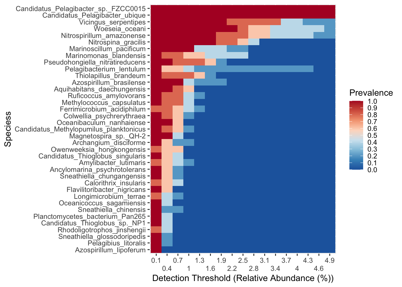
Now Station B !
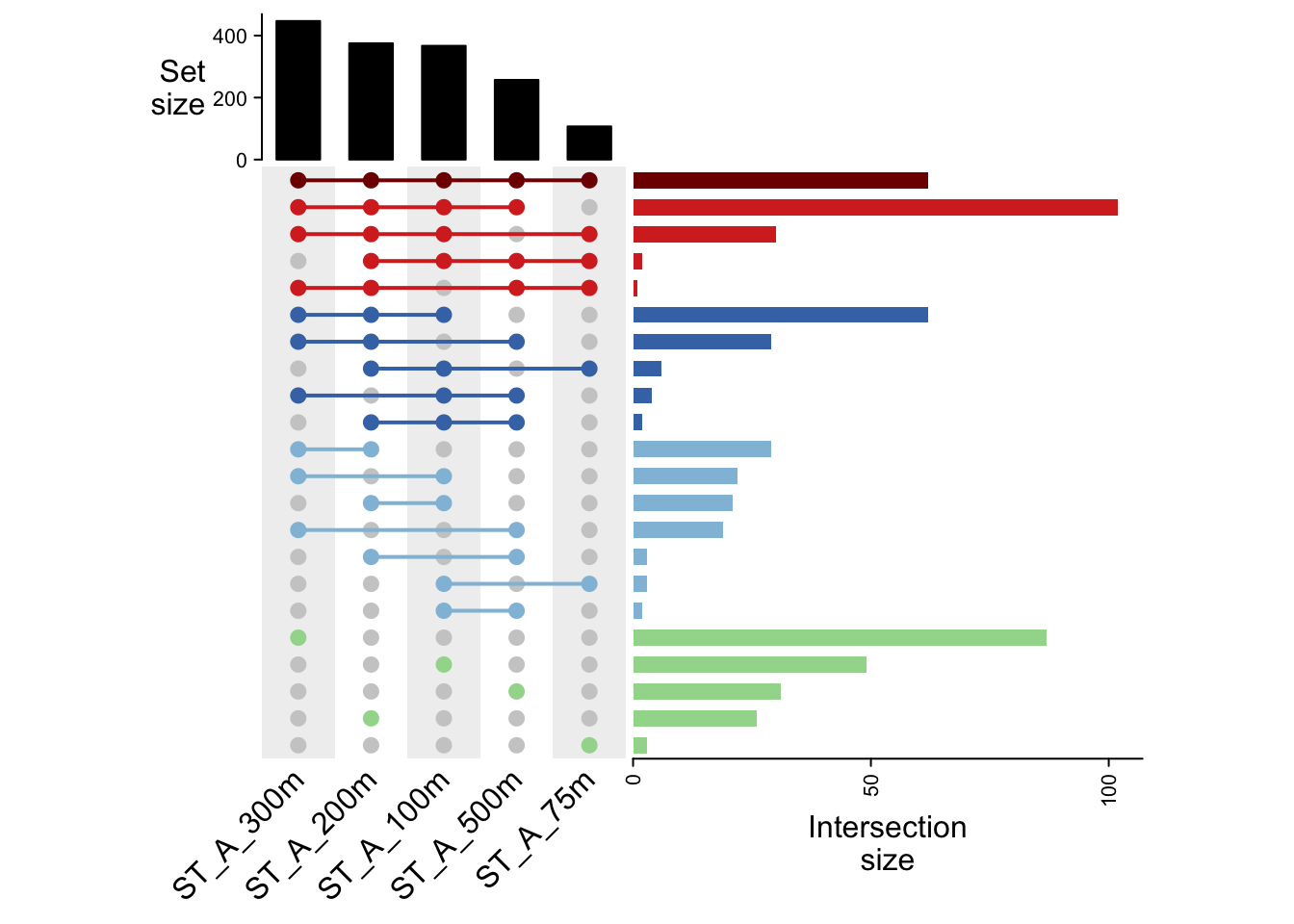
8 Bonus : UpsetPlot
8.1 Matrix OTU table
#recupere table OTU (taxa en ligne!!)
mat <- as(otu_table(sub_StA), "matrix")
8.2 % transformation in Presence/Absence
#trasform en TRUE/FALSE selon >0. Presence/Absence pour l'upsetplot
mat_pa <- mat > 0
head(mat_pa)
barcode13_combine_Q22 barcode14_combine_Q22 barcode22_combine_Q22
1002672 FALSE FALSE FALSE
1002870 TRUE FALSE FALSE
1006 TRUE TRUE TRUE
1008307 TRUE FALSE FALSE
1008392 TRUE TRUE FALSE
102116 FALSE TRUE TRUE
barcode23_combine_Q22 barcode24_combine_Q22
1002672 FALSE TRUE
1002870 TRUE FALSE
1006 TRUE TRUE
1008307 FALSE FALSE
1008392 TRUE TRUE
102116 TRUE TRUE8.3 Change sample labels
#Change les noms samples en ST_A_100 etc
colnames(mat_pa) <- sample_data(sub_StA)$Name
colnames(mat_pa)
[1] "ST_A_300m" "ST_A_500m" "ST_A_75m" "ST_A_100m" "ST_A_200m"8.4 Find all intersection combinations : comb matrix
m <- ComplexHeatmap::make_comb_mat(mat_pa)
m
A combination matrix with 5 sets and 22 combinations.
ranges of combination set size: c(1, 102).
mode for the combination size: distinct.
sets are on rows.
Top 8 combination sets are:
ST_A_300m ST_A_500m ST_A_75m ST_A_100m ST_A_200m code size
x x x x 11011 102
x 10000 87
x x x x x 11111 62
x x x 10011 62
x 00010 49
x 01000 31
x x x x 10111 30
x x x 11001 29
Sets are:
set size
ST_A_300m 447
ST_A_500m 257
ST_A_75m 107
ST_A_100m 367
ST_A_200m 375Transposition for future display in line
m_t <- t(m)8.5 Sort for ideal display
# Trie par degree decroissant, puis par taille decroissante)
comb_order <- base::order(
  -ComplexHeatmap::comb_degree(m_t),
  -ComplexHeatmap::comb_size(m_t)
)
To understand
# Returns the number of sets involved in each combination (how many groups share the same taxa)
ComplexHeatmap::comb_degree(m_t)
11111 11101 11011 10111 01111 11010 11001 10011 01011 00111 11000 10010 10001
5 4 4 4 4 3 3 3 3 3 2 2 2
01010 01001 00110 00011 10000 01000 00100 00010 00001
2 2 2 2 1 1 1 1 1 # Returns the size of each combination (the number of taxa present in each intersection)
ComplexHeatmap::comb_size(m_t)11111 11101 11011 10111 01111 11010 11001 10011 01011 00111 11000 10010 10001
62 1 102 30 2 4 29 62 2 6 19 22 29
01010 01001 00110 00011 10000 01000 00100 00010 00001
2 3 3 21 87 31 3 49 26 # Defines the order in which combinations are displayed (e.g., by degree, size and then by number of taxa within)
comb_order [1] 1 3 4 5 2 8 7 10 6 9 13 12 17 11 15 16 14 18 21 19 22 208.6 Color selection
#Definir des couleurs
comb_cols <- c(
  "1" = "#A1D99B",
  "2" = "#91bfdb",
  "3" = "#4575b4",
  "4" = "#d73027",
  "5" = "#7f0000"
)

comb_col_vec <- comb_cols[as.character(ComplexHeatmap::comb_degree(m_t))]
comb_cols
1 2 3 4 5
"#A1D99B" "#91bfdb" "#4575b4" "#d73027" "#7f0000" 8.7 Final plot
ht <- ComplexHeatmap::UpSet(
  m_t, #matrice des intersections "ronds"
  comb_order = comb_order, # Trie de l'ordre d'apparition qu'on a fait
  comb_col = comb_col_vec, # vecteur couleur qu'on a fait  pour les ronds

  width = unit(50, "mm"), #taille du plot
  pt_size = unit(3, "mm"), # taille des rond

  right_annotation = upset_right_annotation( #barplot a droite
    m_t,
      width = unit(70, "mm"),   #largeur plot a droite
    gp = gpar(fill = comb_col_vec, col = NA), #meme couleur que les ronds, pas de contour
    axis_param = list(side = "bottom")
  ),

  column_names_rot = 45 #angle pour label du bas 45°
)

#Affichage
draw(ht)